🚀 Software Engineering Notes

Welcome to my living collection of software engineering notes.

This book is built as a fast, practical reference for topics I want to review regularly: problem solving, systems and cloud concepts, C++ fundamentals, design patterns, and quantum topics. The goal is simple: keep useful material in one place and make it easy to revisit.

What This Book Is

A study hub for core software engineering topics.
A personal knowledge base that keeps growing over time.
A reader-friendly reference with short sections, examples, formulas, and categorized notes.

Start Here

If you are opening these notes for the first time, these are good entry points:

Quantum Physics
AI + Machine Learning
Object-Oriented Programming
Array / String
Creational Patterns

Explore by Topic

🧠 LeetCode

💻 C++

What to Expect

Concise explanations instead of long textbook-style chapters.
Notes organized by subject so review is fast.
Mathematical notation where needed for physics and quantum sections.
Problem-solving notes grouped by interview pattern.
A structure that favors quick lookup over formal prose.

Best Way to Use These Notes

Use the sidebar to jump between sections.
Use the search to find a concept quickly.
Treat chapters as reference pages, not necessarily linear reading.
Revisit the same topic multiple times and refine your understanding.

Feedback and Contributions

If you spot an error, unclear explanation, or missing topic, contributions and suggestions are welcome.

Credits
License

Quantum Physics

Birth of Quantum Mechanics
Photoelectric Effect and Wave-Particle Duality
Bohr Model of the Atom
Wave Function, Superposition, and Wave Packets
Uncertainty Principle
Schrodinger Equation
Expectation Value

Birth of Quantum Mechanics

Blackbody Radiation

A blackbody is an ideal object that:

Absorbs 100% of incident electromagnetic radiation.
Emits radiation that depends only on its temperature.
Has an emission spectrum independent of its material.

A cavity with a small hole approximates a blackbody because radiation entering the hole undergoes many reflections and is almost completely absorbed before escaping.

Intensity and Spectral Intensity

Total intensity (power per unit area):

\[ I = \frac{E}{A t} \]

Spectral intensity (power per unit area per unit frequency):

\[ I_f = \frac{dE}{dA , dt , df} \]

Total intensity is obtained by integrating over all frequencies:

\[ I = \int_0^\infty I_f , df \]

Temperature Dependence

As temperature increases:

The peak of the spectrum shifts to higher frequency.
The peak wavelength decreases.
The total emitted intensity increases rapidly.

Hotter objects change visible color:

~3000 K → red glow
~6000 K → yellow-white
~12000 K → bluish-white

Wien’s Displacement Law

Peak frequency form:

\[ f_{\text{peak}} = (5.88 \times 10^{10} , \text{Hz/K}) , T \]

Peak wavelength form:

\[ \lambda_{\text{peak}} = \frac{2.90 \times 10^{-3},\mathrm{m\cdot K}}{T} \]

Scaling behavior:

If $T$ doubles → $f_{\text{peak}}$ doubles.
If $T$ doubles → $\lambda_{\text{peak}}$ halves.

Stefan–Boltzmann Law

Total emitted intensity:

\[ I = \sigma T^4 \]

where

\[ \sigma = 5.67 \times 10^{-8},\mathrm{W,m^{-2},K^{-4}} \]

If temperature doubles, total emitted power increases by $2^4 = 16$.

Classical Prediction: Rayleigh–Jeans Law

Classical equipartition assumes each mode has average energy:

\[ E = k_B T \]

Number of modes per unit frequency is proportional to $f^2$.

Rayleigh–Jeans law:

\[ I_f^{RJ}(f,T) = \frac{2 f^2}{c^2} k_B T \]

Total energy prediction:

\[ \int_0^\infty f^2 , df = \infty \]

This divergence at high frequency is called the ultraviolet catastrophe.

Planck’s Quantum Hypothesis

Planck proposed that energy is quantized:

\[ E = n h f, \quad n = 0,1,2,\dots \]

where

\[ h = 6.626 \times 10^{-34},\mathrm{J\cdot s} \]

Average energy per mode becomes:

\[ \langle E \rangle = \frac{h f}{e^{hf/k_B T} - 1} \]

Planck’s radiation law:

\[ I_f(f,T) = \frac{2 f^2}{c^2} \frac{h f}{e^{hf/k_B T} - 1} \]

Why Planck’s Law Resolves the Catastrophe

At high frequency ($hf \gg k_B T$):

\[ e^{hf/k_B T} \gg 1 \]

Thus

\[ \langle E \rangle \rightarrow 0 \]

High-frequency modes are exponentially suppressed, preventing divergence.

Low-Frequency Limit (Classical Recovery)

When $hf \ll k_B T$, use the approximation:

\[ e^{hf/k_B T} \approx 1 + \frac{hf}{k_B T} \]

Substituting:

\[ \langle E \rangle \approx k_B T \]

Planck’s law reduces to the Rayleigh–Jeans result at low frequencies.

Photon Energy

Energy of a single photon:

\[ E = h f \]

Using wavelength:

\[ E = \frac{hc}{\lambda} \]

Key Constants

Planck constant:

\[ h = 6.626 \times 10^{-34},\mathrm{J\cdot s} \]

Boltzmann constant:

\[ k_B = 1.381 \times 10^{-23} , \text{J/K} \]

Speed of light:

\[ c = 3.00 \times 10^8 , \text{m/s} \]

Stefan–Boltzmann constant:

\[ \sigma = 5.67 \times 10^{-8} , \text{W/m}^2\text{K}^4 \]

Conceptual Takeaways

Classical physics fails because it assumes continuous energy.
The number of modes grows with $f^2$, causing divergence.
Quantization suppresses high-frequency energy.
Planck’s law matches experiment at all frequencies.
At low frequency → classical behavior.
At high frequency → quantum behavior dominates.

Photoelectric Effect and Wave-Particle Duality

The Photoelectric Effect

The photoelectric effect occurs when light shines on a metal surface and electrons are ejected.

Key experimental observations:

No electrons are emitted below a certain threshold frequency.
Increasing light intensity increases the number of emitted electrons.
Increasing light frequency increases the kinetic energy of emitted electrons.
Emission occurs instantly, even at low intensity.

These results could not be explained using classical wave theory.

Classical Prediction (Incorrect)

Classical wave theory predicted:

Energy should depend on intensity, not frequency.
Electrons should accumulate energy gradually.
There should be a measurable time delay before emission.

Experiments showed this was completely wrong.

Einstein’s Explanation (1905)

Einstein proposed that light consists of particles called photons.

Each photon carries energy:

\[ E = h f \]

When a photon strikes an electron:

Part of its energy is used to overcome the metal’s work function.
The remainder becomes kinetic energy.

Photoelectric Equation

Energy conservation gives:

\[ h f = W + K_{\text{max}} \]

where:

$W$ = work function (minimum energy needed to remove electron)
$K_{\text{max}}$ = maximum kinetic energy of emitted electrons

Thus:

\[ K_{\text{max}} = h f - W \]

Threshold Frequency

The threshold frequency $f0$ occurs when $K{\text{max}} = 0$:

\[ h f_0 = W \]

So:

\[ f_0 = \frac{W}{h} \]

If $f < f_0$, no electrons are emitted — regardless of intensity.

This was impossible under classical physics.

Experimental Graph

If we plot $K_{\text{max}}$ vs frequency:

\[ K_{\text{max}} = h f - W \]

This is a straight line:

Slope = $h$
Intercept = $-W$
Zero crossing = $f_0$

This experiment allowed direct measurement of Planck’s constant.

Intensity vs Frequency

Intensity controls number of photons → number of electrons emitted
Frequency controls energy per photon → kinetic energy of electrons

Do not confuse these.

Wave–Particle Duality

Blackbody radiation suggested light energy is quantized.

The photoelectric effect showed:

Light behaves like discrete particles.
Energy transfer is localized and instantaneous.

Thus light exhibits particle-like behavior.

But interference experiments show light also behaves like a wave.

Conclusion:

Light has wave–particle duality.

It cannot be described fully as only a wave or only a particle.

Momentum of a Photon

Photons carry momentum even though they have no mass.

Using:

\[ E = p c \]

Since $E = h f$ and $f = \frac{c}{\lambda}$:

\[ p = \frac{h}{\lambda} \]

This will later connect to de Broglie matter waves.

Key Constants

Planck constant:

\[ h = 6.626 \times 10^{-34},\mathrm{J\cdot s} \]

Electron rest mass:

\[ m_e = 9.11 \times 10^{-31},\mathrm{kg} \]

Speed of light:

\[ c = 3.00 \times 10^8,\mathrm{m,s^{-1}} \]

Conceptual Takeaways

Light energy is quantized.
Frequency determines photon energy.
Intensity determines photon number.
Wave and particle descriptions are both necessary.

Bohr Model of the Atom

Atomic Spectra

When atoms are excited, they emit light at discrete wavelengths.

Instead of a continuous spectrum, hydrogen produces sharp spectral lines.

These lines form series:

Lyman series → ultraviolet
Balmer series → visible
Paschen series → infrared

This showed that atomic energy levels are discrete.

The Rydberg Formula

The wavelengths of hydrogen spectral lines follow the Rydberg formula:

\[ \frac{1}{\lambda} = R_H \left( \frac{1}{n_f^2} - \frac{1}{n_i^2} \right) \]

where

$R_H = 1.097 \times 10^7 , \mathrm{m^{-1}}$
$n_i$ = initial energy level
$n_f$ = final energy level

For emission:

\[ n_i > n_f \]

Bohr’s Model (1913)

Niels Bohr proposed a model of the hydrogen atom with three key assumptions:

Electrons move in circular orbits around the nucleus.
Only certain quantized orbits are allowed.
Radiation is emitted only when electrons transition between energy levels.

Quantization of Angular Momentum

Bohr proposed that the electron’s angular momentum is quantized:

\[ m v r = n \hbar \]

where

$n = 1,2,3,\dots$
$\hbar = \frac{h}{2\pi}$

This condition restricts electrons to specific allowed orbits.

Radius of Allowed Orbits

Solving the force balance between Coulomb attraction and centripetal force gives:

\[ r_n = n^2 a_0 \]

where

\[ a_0 = 5.29 \times 10^{-11} , \text{m} \]

is the Bohr radius.

Energy Levels of Hydrogen

The allowed energies of hydrogen are:

\[ E_n = -\frac{13.6 , \text{eV}}{n^2} \]

Properties:

Energy levels become closer together as $n$ increases.
$E = 0$ corresponds to a free electron.

Photon Emission During Transitions

When an electron moves between levels:

\[ \Delta E = E_i - E_f \]

A photon is emitted with energy:

\[ hf = E_i - E_f \]

Thus:

\[ \lambda = \frac{hc}{E_i - E_f} \]

This explains the hydrogen spectral lines.

Connection to de Broglie Waves

The Bohr orbit condition can be interpreted as a standing wave condition:

\[ 2\pi r = n\lambda \]

Only wavelengths that fit an integer number of times around the orbit are allowed.

This links atomic structure to matter waves.

Conceptual Takeaways

Atomic energy levels are quantized.
Spectral lines arise from electron transitions.
Angular momentum is quantized in units of $\hbar$.
Bohr’s model explains hydrogen spectra but fails for multi-electron atoms.

Wave Function, Superposition, and Wave Packets

The Wave Function

Quantum particles are described by a wave function:

\[ \psi(x,t) \]

The wave function contains all information about the particle.

The probability density of finding a particle is:

\[ P(x,t) = |\psi(x,t)|^2 \]

Normalization

Because the particle must exist somewhere:

\[ \int_{-\infty}^{\infty} |\psi(x,t)|^2 dx = 1 \]

This is called the normalization condition.

Plane Waves

A free particle can be described by a plane wave:

\[ \psi(x,t) = A e^{i(kx - \omega t)} \]

where

$k$ = wave number
$\omega$ = angular frequency

Relations:

\[ k = \frac{2\pi}{\lambda} \]

\[ p = \hbar k \]

\[ E = \hbar \omega \]

Superposition of Waves

Quantum wave functions obey the principle of superposition.

If $\psi_1$ and $\psi_2$ are valid solutions, then:

\[ \psi = \psi_1 + \psi_2 \]

is also a valid solution.

Interference between waves produces new spatial structures.

Superposition of Two Waves

Consider two waves:

\[ \psi_1 = A \sin(k_1 x) \]

\[ \psi_2 = A \sin(k_2 x) \]

Their sum is

\[ \psi = 2A \sin(k_{avg} x)\cos\left(\frac{\Delta k}{2}x\right) \]

This creates an envelope that localizes the wave.

Wave Packets

A wave packet is formed by combining many waves with different $k$ values:

\[ \psi(x) = \int g(k)\cos(kx),dk \]

Wave packets represent localized particles.

Properties:

Narrow packet → wide range of $k$
Wide packet → narrow range of $k$

Spatial Localization

The spread in position and wave number satisfies

\[ \Delta x \Delta k \sim 1 \]

Using $p = \hbar k$ gives the basis for the uncertainty principle.

Conceptual Takeaways

The wave function describes probability amplitudes.
Superposition allows interference and localization.
A localized particle corresponds to a wave packet.
Localization requires a range of momenta.

Uncertainty Principle

Position–Momentum Uncertainty

A wave packet cannot have both perfectly defined position and momentum.

The fundamental relation is

\[ \Delta x \Delta p \ge \frac{\hbar}{2} \]

This is the Heisenberg uncertainty principle.

Origin of the Uncertainty Relation

A localized particle requires many wave numbers.

From Fourier analysis:

\[ \Delta x \Delta k \approx \frac{1}{2} \]

Using

\[ p = \hbar k \]

we obtain

\[ \Delta x \Delta p \ge \frac{\hbar}{2} \]

Energy–Time Uncertainty

A similar relation exists for energy and time:

\[ \Delta E \Delta t \gtrsim \frac{\hbar}{2} \]

Short-lived states have large energy uncertainty.

Physical Interpretation

The uncertainty principle does not arise from measurement errors.

Instead it reflects a fundamental property of quantum states.

Key consequences:

A particle cannot have a perfectly defined trajectory.
Confinement increases momentum uncertainty.

Example: Particle in a Nucleus

If a proton is confined to

\[ \Delta x \sim 10^{-15} , \text{m} \]

then

\[ \Delta p \gtrsim \frac{\hbar}{2\Delta x} \]

This implies a large minimum kinetic energy.

Conceptual Takeaways

Position and momentum cannot both be precisely known.
Localization requires a wide momentum distribution.
Quantum uncertainty is negligible for macroscopic objects.

Schrodinger Equation

Operators in Quantum Mechanics

Physical quantities are represented by operators.

Momentum operator:

$$ \hat{p} = -i\hbar \frac{\partial}{\partial x} $$

Energy operator:

$$ \hat{E} = i\hbar \frac{\partial}{\partial t} $$

Time-Dependent Schrödinger Equation

The fundamental equation of quantum mechanics is

\[ i\hbar \frac{\partial \psi}{\partial t} = -\frac{\hbar^2}{2m} \frac{\partial^2 \psi}{\partial x^2} + V(x),\psi \]

where

$m$ = particle mass
$V(x)$ = potential energy

Time-Independent Schrödinger Equation

If the potential does not depend on time:

\[ -\frac{\hbar^2}{2m} \frac{d^2 \psi}{dx^2} + V(x),\psi = E\psi \]

Solutions give the allowed energy levels.

Free Particle

For a free particle:

\[ V(x) = 0 \]

Solutions are plane waves:

$$ \psi = Ae^{ikx} + Be^{-ikx} $$

Energy:

$$ E = \frac{\hbar^2 k^2}{2m} $$

Particle in an Infinite Potential Well

Potential:

$V = 0$ inside the box
$V = \infty$ at the walls

Boundary conditions:

\[ \psi(0) = \psi(L) = 0 \]

Wave functions:

\[ \psi_n(x) = \sqrt{\frac{2}{L}} \sin\left(\frac{n\pi x}{L}\right) \]

Allowed energies:

\[ E_n = \frac{n^2 \pi^2 \hbar^2}{2mL^2} = \frac{n^2 h^2}{8mL^2} \]

Quantum Tunneling

If a particle encounters a barrier with

\[ E < V_0 \]

classically it cannot cross.

Quantum mechanically, the wave function penetrates the barrier.

Transmission probability decreases exponentially with barrier width.

Conceptual Takeaways

Schrödinger’s equation governs quantum dynamics.
Boundary conditions produce quantized energies.
Wave functions determine probability distributions.
Quantum particles can tunnel through barriers.

Expectation Value

Probability Density

The probability density of finding a particle at position $x$ is

\[ P(x) = |\psi(x)|^2 \]

The total probability must equal 1.

Expectation Value of Position

The expectation value of position is

\[ \langle x \rangle = \int_{-\infty}^{\infty} x |\psi(x)|^2 dx \]

This represents the average result of many measurements.

Expectation Value of an Operator

For any observable operator $\hat{O}$:

\[ \langle O \rangle = \int \psi^* \hat{O} \psi , dx \]

Momentum Expectation Value

Using the momentum operator:

\[ \langle \hat{p} \rangle = \int \psi^* \left( -i\hbar \frac{\partial}{\partial x} \right) \psi , dx \]

Energy Expectation Value

Using the energy operator:

\[ \langle \hat{E} \rangle = \int \psi^* \left( i\hbar \frac{\partial}{\partial t} \right) \psi , dx \]

Expectation vs Measurement

Important distinctions:

The expectation value is not the most likely value.
It is the average over many measurements.

Individual measurements may produce different results.

Conceptual Takeaways

Quantum predictions are probabilistic.
The wave function determines measurement statistics.
Expectation values correspond to measurable averages.

Quantum Information

Quantum Interference
Polarization and Wave Plates
Dense Coding
Quantum Teleportation
Entanglement Swapping
Quantum Key Distribution (QKD)

Quantum Interference

Beam Splitter and Superposition

A beam splitter (BS) creates a quantum superposition of paths rather than splitting a photon physically.

For a 50/50 beam splitter:

\[ | \text{in} \rangle \rightarrow \frac{1}{\sqrt{2}} | \text{transmitted} \rangle + \frac{i}{\sqrt{2}} | \text{reflected} \rangle \]

The coefficients are probability amplitudes
Probabilities are obtained by:

\[ P = |\text{amplitude}|^2 \]

Single Beam Splitter Experiment

A photon incident on a beam splitter is detected at one of two detectors:

\[ P(D_1) = P(D_2) = \frac{1}{2} \]

The photon is never split between detectors
This appears as classical randomness

Multiple Paths Without Interference

With multiple beam splitters and independent paths:

\[ P(D_1) = P(D_2) = P(D_3) = P(D_4) = \frac{1}{4} \]

Probabilities distribute evenly
No interference occurs when paths are independent

Mach–Zehnder Interferometer

A Mach–Zehnder interferometer consists of:

Beam splitter (creates superposition)
Mirrors (redirect paths)
Second beam splitter (recombines paths)

Interference of Amplitudes

The total amplitude at a detector is:

\[ A_{\text{total}} = A_1 + A_2 \]

The probability is:

\[ P = |A_1 + A_2|^2 \]

This differs from classical addition:

\[ P \neq |A_1|^2 + |A_2|^2 \]

Example: Perfect Interference

For one detector:

\[ A = \frac{i}{2} + \frac{i}{2} = i \]

\[ P = |i|^2 = 1 \]

For the other detector:

\[ A = \frac{i^2}{2} + \frac{1}{2} = 0 \]

\[ P = 0 \]

Result:

All photons arrive at one detector
No photons arrive at the other

Role of Phase

A phase shift modifies a path:

\[ |\psi\rangle \rightarrow e^{i\phi} |\psi\rangle \]

Total amplitude becomes:

\[ A = A_1 + e^{i\phi} A_2 \]

Interference depends on relative phase
Phase determines constructive or destructive interference

Constructive and Destructive Interference

Constructive interference:

\[ |A_1 + A_2|^2 \text{ is maximized} \]

Destructive interference:

\[ A_1 + A_2 = 0 \]

Conditions for Interference

Interference occurs when:

Paths are indistinguishable
Phases are coherent

Blocking a path removes interference because only one amplitude remains.

Conceptual Takeaways

Quantum systems combine amplitudes, not probabilities
Interference arises from complex phase relationships
A photon behaves as a superposition of paths
Measurement removes interference by destroying coherence

Polarization and Wave Plates

Polarization as a Qubit

Photon polarization is a two-level quantum system:

\[ |H\rangle = \begin{bmatrix} 1 \\ 0 \end{bmatrix}, \quad |V\rangle = \begin{bmatrix} 0 \\ 1 \end{bmatrix} \]

General state:

\[ |\psi\rangle = \alpha |H\rangle + \beta |V\rangle \]

with normalization:

\[ |\alpha|^2 + |\beta|^2 = 1 \]

Jones Vector Representation

Polarization is represented as:

\[ \begin{bmatrix} E_x \\ E_y \end{bmatrix} \]

This encodes:

Amplitude
Relative phase

Linear Polarization

At angle $\theta$:

\[ |\theta\rangle = \begin{bmatrix} \cos\theta \\ \sin\theta \end{bmatrix} \]

Special Polarization States

Diagonal:

\[ |D\rangle = \frac{1}{\sqrt{2}} \begin{bmatrix} 1 \\ 1 \end{bmatrix} \]

Anti-diagonal:

\[ |A\rangle = \frac{1}{\sqrt{2}} \begin{bmatrix} 1 \\ -1 \end{bmatrix} \]

Circular Polarization

Right circular:

\[ |R\rangle = \frac{1}{\sqrt{2}} \begin{bmatrix} 1 \\ i \end{bmatrix} \]

Left circular:

\[ |L\rangle = \frac{1}{\sqrt{2}} \begin{bmatrix} 1 \\ -i \end{bmatrix} \]

Circular polarization arises from a phase difference of $\pm \frac{\pi}{2}$

Polarizing Beam Splitter (PBS)

An optical element that separates light into two orthogonal polarizations:

Transmits $|H\rangle$
Reflects $|V\rangle$

Measurement probabilities:

\[ P(H) = |\alpha|^2, \quad P(V) = |\beta|^2 \]

After measurement, the state collapses to one basis state.

Half-Wave Plate (HWP)

A half-wave plate introduces a phase shift between orthogonal components.

Matrix form:

\[ HWP(\theta) = \begin{bmatrix} \cos 2\theta & \sin 2\theta \\ \sin 2\theta & -\cos 2\theta \end{bmatrix} \]

Important Cases

$\theta = 0^\circ$

\[ HWP = \begin{bmatrix} 1 & 0 \\ 0 & -1 \end{bmatrix} \]

Leaves $|H\rangle$ unchanged
Adds phase $-1$ to $|V\rangle$

$\theta = 45^\circ$

\[ HWP = \begin{bmatrix} 0 & 1 \\ 1 & 0 \end{bmatrix} \]

Swaps $|H\rangle \leftrightarrow |V\rangle$

$\theta = 22.5^\circ$

\[ HWP = \frac{1}{\sqrt{2}} \begin{bmatrix} 1 & 1 \\ 1 & -1 \end{bmatrix} \]

Equivalent to the Hadamard transformation

\[ |H\rangle \rightarrow |D\rangle, \quad |V\rangle \rightarrow |A\rangle \]

Physical Interpretation of HWP

A half-wave plate:

Splits the polarization into two orthogonal components
Introduces a phase difference of $\pi$
Recombines the components

This results in a rotation of polarization.

Key Observations

The transformation depends on $2\theta$, not $\theta$
Wave plates perform unitary operations
They act as quantum gates on polarization states

Conceptual Takeaways

Polarization is a quantum two-level system
Phase determines the difference between linear and circular states
Measurement projects onto a basis and destroys superposition
Wave plates implement controlled transformations of quantum states

Dense Coding

Overview

Dense coding is a quantum communication protocol that allows sending two classical bits by transmitting only one qubit, using a shared entangled pair.

Key idea:

Classical limit: 1 qubit → 1 bit
With entanglement: 1 qubit → 2 bits

Initial Setup

Alice and Bob share an entangled Bell state:

\[ |\Phi^+\rangle = \frac{1}{\sqrt{2}}(|00\rangle + |11\rangle) \]

Ownership:

Alice holds qubit 1
Bob holds qubit 2

This shared entanglement is the key resource.

Bell States

The four maximally entangled Bell states:

\[ |\Phi^+\rangle = \frac{1}{\sqrt{2}}(|00\rangle + |11\rangle) \]

\[ |\Phi^-\rangle = \frac{1}{\sqrt{2}}(|00\rangle - |11\rangle) \]

\[ |\Psi^+\rangle = \frac{1}{\sqrt{2}}(|01\rangle + |10\rangle) \]

\[ |\Psi^-\rangle = \frac{1}{\sqrt{2}}(|01\rangle - |10\rangle) \]

Interpretation:

$ \Phi $: correlated bits (same values)
$ \Psi $: anti-correlated bits (opposite values)
$ + / - $: relative phase difference

Encoding by Alice

Alice encodes 2 classical bits by applying one of four operations to her qubit:

\[ I = \begin{pmatrix} 1 & 0 \\ 0 & 1 \end{pmatrix} \]

\[ X = \begin{pmatrix} 0 & 1 \\ 1 & 0 \end{pmatrix} \]

\[ Z = \begin{pmatrix} 1 & 0 \\ 0 & -1 \end{pmatrix} \]

\[ XZ = \begin{pmatrix} 0 & 1 \\ -1 & 0 \end{pmatrix} \]

Mapping:

Bits	Operation	Resulting State
00	$ I $	$ \|\Phi^+\rangle $
01	$ X $	$ \|\Psi^+\rangle $
10	$ Z $	$ \|\Phi^-\rangle $
11	$ XZ $	$ \|\Psi^-\rangle $

Key idea:

Alice does not send two bits directly
She transforms the shared entangled state

Transmission

After encoding:

Alice sends her qubit to Bob
Bob now has both qubits

Only one qubit is physically transmitted

Decoding by Bob

Bob performs a Bell-state measurement.

Each Bell state corresponds to a unique 2-bit message
If all four states are distinguishable:

\[ I = \log_2(4) = 2 \text{ bits} \]

This exceeds the classical limit.

Information Capacity

Ideal case:

\[ 2 \text{ classical bits per qubit} \]

Classical limit:

\[ 1 \text{ bit per qubit} \]

Entanglement doubles the capacity.

Physical Implementation (Linear Optics)

In practice, photons are used with polarization:

$ |H\rangle $ = horizontal
$ |V\rangle $ = vertical

Bell states become:

\[ |\Phi^+\rangle = \frac{1}{\sqrt{2}}(|HH\rangle + |VV\rangle) \]

\[ |\Phi^-\rangle = \frac{1}{\sqrt{2}}(|HH\rangle - |VV\rangle) \]

\[ |\Psi^+\rangle = \frac{1}{\sqrt{2}}(|HV\rangle + |VH\rangle) \]

\[ |\Psi^-\rangle = \frac{1}{\sqrt{2}}(|HV\rangle - |VH\rangle) \]

Alice’s Encoding with Wave Plates

Alice uses half-wave plates (HWPs):

No HWP → $ |\Psi^+\rangle $
HWP(0°) → phase flip
HWP(45°) → bit flip
Both → combined transformation

These implement the operators $ I, X, Z, XZ $

Bell-State Measurement (BSA)

Bob uses:

Beam splitter (BS)
Polarizing beam splitters (PBS)
Detectors

The measurement outcome depends on photon behavior:

Interference at BS
Polarization splitting at PBS

Key Physical Effects

Bosonic Symmetry

Photons are identical particles:

\[ |H_1 V_2\rangle = |V_2 H_1\rangle \]

This leads to interference effects.

Hong–Ou–Mandel Interference

At a beam splitter:

Some states → photons bunch (same output)
Some states → photons separate (different outputs)

This determines which Bell states can be distinguished.

Detection Patterns

From the Bell-state analyzer:

$ |\Psi^-\rangle $: photons exit different ports
$ |\Psi^+\rangle $: same port, different detectors
$ |\Phi^\pm\rangle $: same detector pattern

Key limitation:

Cannot distinguish $ |\Phi^+\rangle $ vs $ |\Phi^-\rangle $

Practical Limitation

Linear optics cannot fully distinguish all Bell states.

Result:

Only 3 distinguishable outcomes

\[ I_{\text{max}} = \log_2(3) \approx 1.58 \text{ bits} \]

Improved Bell-State Analyzer

Using auxiliary entangled photons:

Near-deterministic discrimination
$ \sim 75% $ success rate

Still limited by linear optics constraints.

Conceptual Takeaways

Entanglement enables higher communication capacity
Information is encoded in global quantum states, not local bits
Alice modifies a shared state, not her qubit alone
Measurement requires joint operations on both qubits
Physical implementations impose real limitations

Common Misconceptions

Alice does not “store two bits in one qubit”
Bob cannot decode without receiving Alice’s qubit
Entanglement alone does not transmit information
Without entanglement → dense coding is impossible

Quantum Teleportation

Overview

Quantum teleportation is a protocol that transfers an unknown quantum state from one location to another using:

Entanglement
Classical communication

Key idea:

The quantum state is not copied
The original is destroyed
The state is reconstructed at the destination

The Problem

Given an unknown qubit:

\[ |\psi\rangle = \alpha|0\rangle + \beta|1\rangle \]

Goal:

\[ |\psi\rangle_A \rightarrow |\psi\rangle_B \]

Naively, one might try:

\[ |\psi\rangle |0\rangle \rightarrow |\psi\rangle |\psi\rangle \]

This is impossible.

No-Cloning Theorem

Unknown quantum states cannot be copied.

Reason:

Linearity implies:

\[ C(\alpha|0\rangle + \beta|1\rangle) = \alpha C|0\rangle + \beta C|1\rangle \]

But cloning would require:

\[ (\alpha|0\rangle + \beta|1\rangle)(\alpha|0\rangle + \beta|1\rangle) \]

These expressions are not equal for general $ \alpha, \beta $.

Conclusion:

Cloning is impossible
State must be transferred, not duplicated

Initial Setup

Three qubits:

Qubit 1: unknown state $ |\psi\rangle $ (Alice)
Qubit 2: entangled (Alice)
Qubit 3: entangled (Bob)

Shared Bell state:

\[ |\Phi^+\rangle_{23} = \frac{1}{\sqrt{2}}(|00\rangle + |11\rangle) \]

Ownership:

Alice → qubits 1 and 2
Bob → qubit 3

Total Initial State

\[ |\Psi\rangle = |\psi\rangle_1 \otimes |\Phi^+\rangle_{23} \]

\[ = (\alpha|0\rangle + \beta|1\rangle) \frac{1}{\sqrt{2}}(|00\rangle + |11\rangle) \]

This is a three-qubit system.

Bell States

\[ |\Phi^\pm\rangle = \frac{1}{\sqrt{2}}(|00\rangle \pm |11\rangle) \]

\[ |\Psi^\pm\rangle = \frac{1}{\sqrt{2}}(|01\rangle \pm |10\rangle) \]

These form a complete basis for two qubits.

Bell Basis Expansion

The total state can be rewritten as:

\[ |\Psi\rangle = \frac{1}{2} \Big(|\Phi^+\rangle_{12} (\alpha|0\rangle + \beta|1\rangle)_3 - |\Phi^-\rangle_{12} (\alpha|0\rangle - \beta|1\rangle)_3 - |\Psi^+\rangle_{12} (\alpha|1\rangle + \beta|0\rangle)_3 - |\Psi^-\rangle_{12} (\alpha|1\rangle - \beta|0\rangle)_3\Big) \]

Key insight:

Alice’s measurement outcome determines Bob’s state

Measurement by Alice

Alice performs a Bell-state measurement on qubits 1 and 2.

Result:

One of four Bell states
Produces 2 classical bits

After measurement:

Original state is destroyed
Bob’s qubit collapses into a related state

Conditional States at Bob

Alice Outcome	Bob’s State
$ \|\Phi^+\rangle $	$ \alpha\|0\rangle + \beta\|1\rangle $
$ \|\Phi^-\rangle $	$ \alpha\|0\rangle - \beta\|1\rangle $
$ \|\Psi^+\rangle $	$ \alpha\|1\rangle + \beta\|0\rangle $
$ \|\Psi^-\rangle $	$ \alpha\|1\rangle - \beta\|0\rangle $

Bob has a modified version of $ |\psi\rangle $.

Classical Communication

Alice sends 2 classical bits to Bob.

Important:

Without this, Bob cannot recover the state
No faster-than-light communication

Correction by Bob

Bob applies an operation depending on Alice’s result:

Bits	Operation
00	$ I $
01	$ Z $
10	$ X $
11	$ XZ $

After correction:

\[ |\psi\rangle_B = \alpha|0\rangle + \beta|1\rangle \]

Final Result

Bob obtains the original quantum state
Alice’s state is destroyed

\[ |\psi\rangle_A \rightarrow |\psi\rangle_B \]

No duplication occurs.

Physical Implementation (Optical Systems)

Qubits represented by polarization:

$ |H\rangle $ = horizontal
$ |V\rangle $ = vertical

Components:

Beam splitter (BS)
Polarizing beam splitters (PBS)
Detectors

Bell-state analyzer:

Can distinguish only some Bell states

Practical Limitation

Linear optics can distinguish:

\[ |\Psi^+\rangle, \quad |\Psi^-\rangle \]

But not:

\[ |\Phi^+\rangle, \quad |\Phi^-\rangle \]

Result:

\[ P_{\text{success}} = \frac{1}{2} \]

Teleportation is probabilistic in practice.

Conceptual Flow

Entanglement shared
Alice entangles unknown with Bell pair
Alice measures (destroys original state)
Classical bits sent to Bob
Bob applies correction
State reconstructed

Conceptual Takeaways

Quantum information cannot be copied
Entanglement enables state transfer
Classical communication is required
Information is transferred, not particles
Measurement redistributes quantum information

Common Misconceptions

Teleportation does not move matter
Entanglement alone does not transmit information
The state does not exist in two places
Classical communication is essential

Entanglement Swapping

Overview

Entanglement swapping is a protocol that creates entanglement between two particles that have never interacted.

Key idea:

Two independent entangled pairs are prepared
A joint measurement is performed on one particle from each pair
This creates entanglement between the remaining two particles

Initial Setup

Two Bell pairs:

\[ |\Phi^+\rangle_{12} = \frac{1}{\sqrt{2}}(|00\rangle + |11\rangle) \]

\[ |\Phi^+\rangle_{34} = \frac{1}{\sqrt{2}}(|00\rangle + |11\rangle) \]

Ownership:

Alice → qubit 1
Bob → qubit 4
Middle station → qubits 2 and 3

Initially:

(1,2) are entangled
(3,4) are entangled
(1,4) are not entangled

Total Initial State

\[ |\Psi\rangle = |\Phi^+\rangle_{12} \otimes |\Phi^+\rangle_{34} \]

\[ = \frac{1}{2} (|0000\rangle + |0011\rangle + |1100\rangle + |1111\rangle) \]

This is a four-qubit system.

Bell States

\[ |\Phi^\pm\rangle = \frac{1}{\sqrt{2}}(|00\rangle \pm |11\rangle) \]

\[ |\Psi^\pm\rangle = \frac{1}{\sqrt{2}}(|01\rangle \pm |10\rangle) \]

These form a complete basis for two qubits.

Bell Basis Expansion (Key Step)

Rewrite the total state in terms of Bell states of qubits (2,3):

\[ |\Psi\rangle = \frac{1}{2} \Big( |\Phi^+\rangle_{23} |\Phi^+\rangle_{14} + |\Phi^-\rangle_{23} |\Phi^-\rangle_{14} + |\Psi^+\rangle_{23} |\Psi^+\rangle_{14} + |\Psi^-\rangle_{23} |\Psi^-\rangle_{14} \Big) \]

Key insight:

The system is a superposition of correlated Bell states
Each Bell state of (2,3) is paired with the same Bell state of (1,4)

Measurement at the Middle Station

A Bell-state measurement is performed on qubits 2 and 3.

Result:

One of four Bell states is obtained
The system collapses to the corresponding term

After measurement:

Original entanglement (1–2 and 3–4) is destroyed

Resulting State of (1,4)

Depending on the measurement outcome:

Measurement (2,3)	Resulting State (1,4)
$ \| \Phi^+\rangle $	$ \| \Phi^+\rangle $
$ \| \Phi^-\rangle $	$ \| \Phi^-\rangle $
$ \| \Psi^+\rangle $	$ \| \Psi^+\rangle $
$ \| \Psi^-\rangle $	$ \| \Psi^-\rangle $

Result:

Qubits (1,4) become entangled
Type of entanglement depends on measurement outcome

Classical Communication (Optional Correction)

If a specific Bell state is required:

Measurement result must be sent to Alice or Bob
A correction operation can be applied

This is similar to teleportation:

Operations: $ I, X, Z, XZ $

Final Result

\[ (1,2), (3,4) ;\rightarrow; (1,4) \]

Entanglement is transferred
Qubits 1 and 4 are now entangled
They never interacted directly

Physical Interpretation

Entanglement is not a local property
It is a property of the global quantum state

Measurement:

Does not create entanglement
It selects one correlation pattern already present

Physical Implementation (Optical Systems)

Qubits represented by polarization:

$ |H\rangle $, $ |V\rangle $

Procedure:

Two entangled photon pairs are generated
Photons 2 and 3 interfere at a beam splitter
A Bell-state measurement is performed

Practical Limitation

Linear optics:

Cannot distinguish all Bell states

Typically distinguishable:

\[ |\Psi^+\rangle, \quad |\Psi^-\rangle \]

Result:

\[ P_{\text{success}} = \frac{1}{2} \]

Entanglement swapping is probabilistic in practice.

Conceptual Flow

Prepare two entangled pairs
Bring qubits (2,3) together
Rewrite system in Bell basis
Perform Bell-state measurement on (2,3)
Collapse system to one term
Qubits (1,4) become entangled

Conceptual Takeaways

Entanglement can be created between non-interacting particles
Measurement redistributes quantum correlations
Entanglement is a global property
Basis choice determines how correlations are revealed
Essential for quantum communication networks

Common Misconceptions

Measurement creates entanglement (it does not)
Particles must interact to become entangled
Entanglement is stored locally in particles
The process transmits information instantly

Quantum Key Distribution

Overview

Quantum Key Distribution (QKD) is a method for securely sharing a secret key between two parties using quantum mechanics.

Key idea:

Security is based on physical laws, not computational hardness
Measurement of quantum states disturbs them
Eavesdropping can be detected

Classical Motivation

The one-time pad provides perfect secrecy:

\[ C = M \oplus K \]

$ M $: message
$ K $: secret key
$ C $: ciphertext

Problem:

Alice and Bob must already share a secure key
Key distribution is difficult

QKD addresses this problem by enabling Alice and Bob to establish a shared secret key whose security is guaranteed by quantum mechanics, provided they already share an authenticated public classical channel; in other words, QKD reduces the key-distribution problem to authentication rather than eliminating all trust assumptions.

Quantum Advantage

Two fundamental principles:

No-Cloning Theorem

Unknown quantum states cannot be copied.

Measurement Disturbance

Measuring a quantum state generally changes it.

Conclusion:

An eavesdropper cannot observe communication without being detected

BB84 Protocol

Alice uses two orthogonal bases:

Rectilinear Basis (+)

\[ |0\rangle = |H\rangle, \quad |1\rangle = |V\rangle \]

Diagonal Basis (×)

\[ |0\rangle = |D\rangle, \quad |1\rangle = |A\rangle \]

Basis Relationship

The bases are related by superposition:

\[ |D\rangle = \frac{1}{\sqrt{2}}(|H\rangle + |V\rangle) \]

\[ |A\rangle = \frac{1}{\sqrt{2}}(|H\rangle - |V\rangle) \]

Key consequence:

Measuring in the wrong basis gives random results

Protocol Steps

Alice generates random bits
Alice randomly chooses a basis (+ or ×)
Alice sends encoded qubits
Bob randomly chooses measurement bases
Bob measures each qubit

Measurement Outcomes

Same basis → deterministic result
Different basis → random result (50/50)

Sifting Process

After transmission:

Alice and Bob publicly announce bases only
They discard all mismatched cases

Result:

Remaining bits form the sifted key

Key Efficiency

Approximately:

\[ 50% \text{ of bits are discarded} \]

Eavesdropping (Intercept-Resend Attack)

Eve:

Intercepts qubit
Measures in random basis
Resends qubit

Effect of Eavesdropping

If Eve uses the wrong basis:

She disturbs the state
Bob may receive incorrect value

Even when:

Alice and Bob use the same basis

This introduces errors.

Error Detection

Alice and Bob:

Reveal a subset of bits
Compare results

If error rate is high:

Eavesdropping is detected
Key is discarded

Key Insight

Security arises because:

Information gain ⇒ disturbance
Disturbance ⇒ detectable errors

B92 Protocol

B92 is a simplified QKD protocol using:

Only two non-orthogonal states

Encoding

Alice sends:

Bit 0 → $ |H\rangle $
Bit 1 → $ |D\rangle $

These states are not orthogonal:

\[ \langle H | D \rangle \neq 0 \]

Measurement Bases

Bob randomly measures in:

H/V basis
D/A basis

Measurement Behavior

If Alice sends $ |H\rangle $

H/V → always H
D/A → random

If Alice sends $ |D\rangle $

D/A → always D
H/V → random

Conclusive vs Inconclusive Results

A result is conclusive if it rules out one possibility.

Conclusive Results

Detect V → must be $ |D\rangle $ → bit = 1
Detect A → must be $ |H\rangle $ → bit = 0

Inconclusive Results

Detect H or D → cannot determine bit → discard

Sifting Process

Bob:

Announces positions of conclusive results

Alice:

Keeps corresponding bits

Result:

Shared secret key

Efficiency

Many measurements are discarded
Lower efficiency than BB84

Key Insight

Security arises from:

Inability to perfectly distinguish non-orthogonal states

Conceptual Comparison

Feature	BB84	B92
States used	4	2
Bases	2	implicit
Efficiency	higher	lower
Core principle	basis mismatch	non-orthogonality

Conceptual Takeaways

Quantum mechanics enables secure key distribution
Measurement disturbs quantum states
Eavesdropping introduces detectable errors
BB84 uses basis incompatibility
B92 uses non-orthogonal states
Security is physical, not computational

Common Misconceptions

Randomness alone provides security
QKD transmits the key directly (it generates it)
Eavesdropping can be hidden without errors
Non-orthogonal states can be perfectly distinguished

Quantum Computation

Quantum Gates
Quantum Teleportation Circuit
Superdense Coding Circuit

Quantum Gates

Quantum gates are the fundamental operations of quantum computation.
They act on qubits and are represented as unitary matrices.

A quantum state is a vector
A gate is a matrix
Evolution is matrix multiplication

\[ |\psi’\rangle = U |\psi\rangle \]

Unlike classical gates:

Quantum gates are reversible
They operate on probability amplitudes, not bits

Single-Qubit Gates

Basis States

A single qubit is represented as:

\[ |0\rangle = \begin{bmatrix} 1 \\ 0 \end{bmatrix}, \quad |1\rangle = \begin{bmatrix} 0 \\ 1 \end{bmatrix} \]

A general state:

\[ |\psi\rangle = \alpha |0\rangle + \beta |1\rangle \]

with:

\[ |\alpha|^2 + |\beta|^2 = 1 \]

Pauli-X Gate (NOT Gate)

\[ X = \begin{bmatrix} 0 & 1 \\ 1 & 0 \end{bmatrix} \]

\[ X|0\rangle = |1\rangle, \quad X|1\rangle = |0\rangle \]

Flips the qubit
Equivalent to classical NOT

Pauli-Z Gate (Phase Flip)

\[ Z = \begin{bmatrix} 1 & 0 \\ 0 & -1 \end{bmatrix} \]

\[ Z|0\rangle = |0\rangle, \quad Z|1\rangle = -|1\rangle \]

Does not change probabilities
Changes phase

Hadamard Gate

\[ H = \frac{1}{\sqrt{2}} \begin{bmatrix} 1 & 1 \\ 1 & -1 \end{bmatrix} \]

\[ H|0\rangle = \frac{1}{\sqrt{2}}(|0\rangle + |1\rangle) \]

\[ H|1\rangle = \frac{1}{\sqrt{2}}(|0\rangle - |1\rangle) \]

Creates superposition
Converts deterministic states into probabilistic ones

Measurement and Probability

Measurement outcomes are determined by amplitudes:

\[ P(0) = |\alpha|^2, \quad P(1) = |\beta|^2 \]

Example:

\[ |\psi\rangle = \frac{1}{\sqrt{2}}(|0\rangle + |1\rangle) \]

\[ P(0) = P(1) = \frac{1}{2} \]

Phase Factors

Quantum states can acquire a phase:

\[ |\psi\rangle \rightarrow e^{i\theta} |\psi\rangle \]

Special cases:

\[ e^{i\pi} = -1, \quad e^{i\pi/2} = i \]

Global phase: no physical effect
Relative phase: affects interference and measurement

Gate Composition

Multiple gates are applied in sequence:

\[ U_2 U_1 |\psi\rangle \]

Order matters:

\[ ZX|0\rangle \neq XZ|0\rangle \]

Multi-Qubit Systems

Tensor Product

Multiple qubits are combined using the tensor product:

\[ |a\rangle \otimes |b\rangle \]

Example:

\[ |0\rangle \otimes |0\rangle = |00\rangle = \begin{bmatrix} 1 \\ 0 \\ 0 \\ 0 \end{bmatrix} \]

General rule:

\[ \begin{bmatrix} a \\ b \end{bmatrix} \otimes \begin{bmatrix} c \\ d \end{bmatrix} = \begin{bmatrix} ac \\ ad \\ bc \\ bd \end{bmatrix} \]

Multi-Qubit States

Two-qubit basis states:

$|00\rangle$
$|01\rangle$
$|10\rangle$
$|11\rangle$

These form a 4-dimensional vector space.

Multi-Qubit Gates

CNOT Gate

The Controlled-NOT gate flips the target qubit if the control qubit is 1.

\[ \text{CNOT} |00\rangle = |00\rangle \] \[ \text{CNOT} |01\rangle = |01\rangle \] \[ \text{CNOT} |10\rangle = |11\rangle \] \[ \text{CNOT} |11\rangle = |10\rangle \]

Essential for entanglement
Combines classical control with quantum behavior

SWAP Gate

Swaps two qubits:

\[ |00\rangle \rightarrow |00\rangle \]

\[ |01\rangle \rightarrow |10\rangle \]

\[ |10\rangle \rightarrow |01\rangle \]

\[ |11\rangle \rightarrow |11\rangle \]

Exchanges quantum states
Often implemented using multiple CNOT gates

Controlled-Z Gate (CZ)

Applies a phase flip when both qubits are 1:

\[ |00\rangle \rightarrow |00\rangle \]

\[ |01\rangle \rightarrow |01\rangle \]

\[ |10\rangle \rightarrow |10\rangle \]

\[ |11\rangle \rightarrow -|11\rangle \]

Does not change bit values
Changes phase relationships

Parameterized Gates

Rotation Gate (Rx)

\[ R_x(\theta) = \begin{bmatrix} \cos(\theta/2) & -i\sin(\theta/2) \\ -i\sin(\theta/2) & \cos(\theta/2) \end{bmatrix} \]

Represents rotation around the x-axis
Generalizes discrete gates into continuous operations

General U Gate

\[ U(\theta, \phi, \lambda) \]

Most general single-qubit gate
Can represent all rotations

Special cases:

$U(\theta, 0, 0) = R_y(\theta)$
$U(\theta, -\pi/2, \pi/2) = R_x(\theta)$

Key Takeaways

Quantum gates are unitary matrix operations
Qubits evolve via linear algebra
Measurement depends on probability amplitudes
Tensor products define multi-qubit systems
CNOT enables entanglement
Phase plays a critical role in quantum behavior
Gate order matters — operations are not commutative

Quantum Teleportation Circuit

Quantum teleportation is a protocol that transfers an unknown quantum state from Alice to Bob using:

Entanglement
Classical communication
Quantum gates

The original qubit is destroyed, and the state is reconstructed at Bob’s location.

\[ |\psi\rangle = \alpha |0\rangle + \beta |1\rangle \]

Goal:

\[ |\psi\rangle_A \rightarrow |\psi\rangle_B \]

Circuit Overview

The teleportation circuit consists of three qubits:

Top wire: unknown state $|\psi\rangle$
Middle wire: Alice’s entangled qubit
Bottom wire: Bob’s entangled qubit

Key stages:

Create entanglement (EPR pair)
Perform Bell measurement (Alice)
Send classical bits
Apply correction (Bob)

The protocol uses:

Hadamard (H)
CNOT
Measurement
Conditional gates (X, Z)

Step-by-Step Process

Step 1: Create Entanglement (EPR Pair)

Alice and Bob share a Bell state:

\[ |\Psi^+\rangle = \frac{1}{\sqrt{2}}(|01\rangle + |10\rangle) \]

Created using:

Hadamard on one qubit
CNOT gate

This entanglement is the resource that enables teleportation.

Step 2: Combine with Unknown State

The full system becomes:

\[ |\psi\rangle \otimes |\Psi^+\rangle \]

This expands into a superposition of Bell states:

\[ |\psi\rangle \otimes |\Psi^+\rangle = \frac{1}{2}( |00\rangle (\alpha|0\rangle + \beta|1\rangle) + |01\rangle (\alpha|1\rangle + \beta|0\rangle) + |10\rangle (\alpha|0\rangle - \beta|1\rangle) + |11\rangle (\alpha|1\rangle - \beta|0\rangle) ) \]

Key idea:

The unknown state is now distributed across all three qubits

Step 3: Bell Measurement (Alice)

Alice applies:

CNOT (between her qubits)
Hadamard

Then measures both qubits.

Result:

\[ \frac{1}{2}( |00\rangle (\alpha|0\rangle + \beta|1\rangle) + |01\rangle (\alpha|1\rangle + \beta|0\rangle) + |10\rangle (\alpha|0\rangle - \beta|1\rangle) + |11\rangle (\alpha|1\rangle - \beta|0\rangle) ) \]

Key idea:

Measurement collapses the system into one of four cases.

Bell States and Measurement

Alice’s measurement yields:

$|00\rangle$
$|01\rangle$
$|10\rangle$
$|11\rangle$

Each corresponds to a different transformation of Bob’s qubit.

Important:

Bob’s qubit is already close to $|\psi\rangle$ — just modified by a known operation.

Classical Communication and Correction

Alice sends 2 classical bits to Bob.

Based on the result, Bob applies:

Measurement	Operation
00	Identity
01	X
10	Z
11	XZ

After correction:

\[ |\psi\rangle = \alpha|0\rangle + \beta|1\rangle \]

Bob now has the exact original state.

Key Insights

1. No Faster-Than-Light Communication

Classical bits are required
Teleportation is not instantaneous communication

2. State is Not Copied

The original qubit is destroyed during measurement
This obeys the no-cloning theorem

3. Entanglement is a Resource

Without entanglement, teleportation is impossible
It enables non-local correlations

4. Measurement Drives the Protocol

Measurement collapses the system
Converts quantum information into classical bits

5. Corrections Recover the State

Bob’s qubit is always one operation away from $|\psi\rangle$
Classical information tells him which one

Conceptual Takeaways

Teleportation = entanglement + measurement + classical control
Information is transferred without moving the particle
Quantum states behave as global systems, not local objects

Superdense Coding Circuit

Superdense coding allows Alice to send 2 classical bits to Bob by transmitting only 1 qubit, using shared entanglement.

This is only possible because of entanglement as a resource.

The protocol works by encoding classical information into quantum states.

Protocol Overview

Alice and Bob share an entangled Bell pair
Alice encodes 2 classical bits using a quantum gate
Alice sends her qubit to Bob
Bob performs a joint measurement to recover the 2 bits

Step 1: Entanglement Preparation

Start with:

\[ |00\rangle \]

Apply:

Hadamard on first qubit
CNOT (control = first, target = second)

Result:

\[ |\Phi^+\rangle = \frac{1}{\sqrt{2}} (|00\rangle + |11\rangle) \]

This shared Bell state is distributed between Alice and Bob.

Step 2: Alice Encoding

Alice encodes two classical bits by applying one of four operations to her qubit:

Bits	Operation	Resulting State
00	$I$	$ \|\Phi^+\rangle $
01	$X$	$ \|\Psi^+\rangle $
10	$Z$	$ \|\Phi^-\rangle $
11	$Y$	$ \|\Psi^-\rangle $

Each operation maps the shared state to a different Bell state

Key idea:

Alice is not sending bits directly—she is transforming entanglement

Step 3: Bob Decoding

After receiving Alice’s qubit, Bob performs:

CNOT
Hadamard (on first qubit)

This transforms Bell states into computational basis states:

Then Bob measures and recovers the two classical bits.

Bell States and Encoding

The four Bell states:

\[ |\Phi^+\rangle = \frac{1}{\sqrt{2}}(|00\rangle + |11\rangle) \]

\[ |\Phi^-\rangle = \frac{1}{\sqrt{2}}(|00\rangle - |11\rangle) \]

\[ |\Psi^+\rangle = \frac{1}{\sqrt{2}}(|01\rangle + |10\rangle) \]

\[ |\Psi^-\rangle = \frac{1}{\sqrt{2}}(|01\rangle - |10\rangle) \]

Each represents a distinct global state.

Information Gain

Classically:

1 bit per bit sent

Quantum (superdense coding):

2 bits per qubit

\[ \log_2(4) = 2 \text{ bits} \]

However:

In real systems (e.g., linear optics), not all Bell states are distinguishable
Practical limit ≈ 1.58 bits per qubit

Key Insights

1. Entanglement Enables Compression

Information is encoded into global correlations
Not into a single qubit alone

2. Alice Does Not Send Two Bits Directly

She modifies her half of an entangled state
The message exists in the joint system

3. Bob Needs Both Qubits

Without Alice’s qubit, Bob cannot decode anything
Without prior entanglement, protocol fails

4. This is the Reverse of Teleportation

Teleportation: send 1 qubit using 2 classical bits
Superdense coding: send 2 classical bits using 1 qubit

Conceptual Takeaways

Quantum information can be compressed into entanglement
Operations on one qubit affect the entire system
Measurement extracts classical information from quantum correlations

AI + Machine Learning

Azure Machine Learning
Azure AI Services
Azure AI Foundry
Azure OpenAI Service
Azure AI Search

Azure Machine Learning

Purpose: Provides an end-to-end machine learning platform for data scientists and developers.
Key Capabilities:
- Model training, deployment, and management.
- Automated Machine Learning (AutoML) for no-code/low-code solutions.
- Integration with popular frameworks such as TensorFlow, PyTorch, and Scikit-learn.
Typical Use Cases:
- Predictive analytics
- Fraud detection
- Recommendation systems

Azure AI Services

Purpose: Collection of AI-based services for vision, speech, language understanding, and more.
Key Capabilities:
- Cognitive Services for text analytics, speech-to-text, image recognition, etc.
- Prebuilt AI models for language translation, anomaly detection, sentiment analysis.
Typical Use Cases:
- Chatbots and virtual assistants
- Document processing and OCR
- Audio/video transcription

Azure AI Foundry

Purpose: Helps organizations build, deploy, and operationalize AI solutions rapidly.
Key Capabilities:
- Collaborative environment for data science teams.
- Accelerators and industry-specific solution templates.
- End-to-end MLOps to streamline AI solution lifecycle.
Typical Use Cases:
- Data science collaboration
- Rapid AI prototyping
- Automated CI/CD for AI projects

Azure OpenAI Service

Purpose: Provides access to advanced language models (e.g., GPT series) for building AI solutions.
Key Capabilities:
- Natural language processing (NLP) and generation.
- Code generation, text summarization, translation, etc.
- Easily integrates with other Azure services for end-to-end solutions.
Typical Use Cases:
- Chatbots with contextual awareness
- Intelligent document analysis
- Code completion or generation

Azure AI Search

Purpose: Intelligent search and indexing service powered by AI.
Key Capabilities:
- Natural language processing search queries.
- Cognitive skills for image, OCR, and text analytics.
- Synonym search and ranking capabilities.
Typical Use Cases:
- Website and application content search
- Enterprise data search with AI-driven insights
- E-commerce product search

Compute

Azure Virtual Machines
Azure Virtual Machine Scale Sets
Azure App Service
Azure Kubernetes Service (AKS)
Azure Virtual Desktop
Azure Functions
Azure Container Instances (ACI)
Azure Batch

Azure Virtual Machines

Purpose: On-demand, scalable computing resources in the cloud.
Key Capabilities:
- Wide range of VM sizes, regions, and OS options (Windows, Linux).
- Support for custom images and templates.
- Integration with Virtual Networks, storage, and other Azure services.
Typical Use Cases:
- Lift-and-shift of existing applications to the cloud.
- Development and testing environments.
- Host custom software and workloads.

Azure Virtual Machine Scale Sets

Purpose: Automatically scale virtual machines to handle demand changes.
Key Capabilities:
- Automatic VM provisioning and de-provisioning.
- Load balancing integrations.
- Uniform or flexible orchestration modes.
Typical Use Cases:
- Large-scale compute clusters.
- Stateless web tiers with variable traffic.
- Big data and containerized workloads.

Azure App Service

Purpose: Fully managed platform for building, deploying, and scaling web apps and APIs.
Key Capabilities:
- Supports multiple languages and frameworks (e.g., .NET, Node.js, Python, Java).
- Continuous integration and deployment (CI/CD).
- Built-in autoscaling, monitoring, and security features.
Typical Use Cases:
- Enterprise web applications
- RESTful API hosting
- Minimal management overhead for web deployments

Azure Kubernetes Service (AKS)

Purpose: Managed Kubernetes service to run containerized applications at scale.
Key Capabilities:
- Automated provisioning and cluster management.
- Integration with Azure Container Registry (ACR) for container images.
- Autoscaling, rolling updates, and built-in monitoring.
Typical Use Cases:
- Microservices-based architectures.
- Container orchestration for development and production.
- Hybrid and multi-cloud strategies (with Azure Arc).

Azure Virtual Desktop

Purpose: Provide Windows 10/11 desktops and apps in the cloud.
Key Capabilities:
- Multi-session Windows 10/11 environment.
- Optimizations for Microsoft 365 Apps.
- Integration with Azure Active Directory (Microsoft Entra ID).
Typical Use Cases:
- Remote work scenarios.
- Secure access to corporate desktops and applications.
- Disaster recovery for on-premises desktop environments.

Azure Functions

Purpose: Serverless compute platform for event-driven, on-demand code execution.
Key Capabilities:
- Pay-per-execution billing model (consumption plan).
- Triggers and bindings to integrate with other Azure services.
- Built-in scaling and managed infrastructure.
Typical Use Cases:
- Real-time file processing
- IoT data processing
- Webhooks and microservices

Azure Container Instances (ACI)

Purpose: Run containers without managing servers or clusters.
Key Capabilities:
- Fast, isolated compute for containerized workloads.
- Per-second billing.
- Integrates with Virtual Networks for secure deployments.
Typical Use Cases:
- Batch processing
- Test and development containers
- Event-driven container workloads

Azure Batch

Purpose: Large-scale parallel and high-performance computing (HPC) in the cloud.
Key Capabilities:
- Automatically manage and scale compute nodes.
- Integration with Azure Storage for input/output data.
- Supports Docker containers and common HPC frameworks.
Typical Use Cases:
- Rendering 3D images or simulations
- Financial risk modeling
- Genomic and scientific research

Management and Governance

Azure Subscriptions
Azure Management Groups
Azure Policy
Azure Blueprints
Azure Resource Groups
Azure Tags
Azure Arc
Azure Resource Manager (ARM) Templates
Azure Purview
Azure Advisor

Azure Subscriptions

Purpose: Logical container for Azure resources, billing, and usage.
Key Capabilities:
- Payment and billing boundary.
- Resource access and usage quotas.
- Linked to Azure Active Directory tenant.
Typical Use Cases:
- Organizing workloads by department or project.
- Enforcing budgetary constraints and spending thresholds.

Azure Management Groups

Purpose: Hierarchical grouping of subscriptions for organizational governance.
Key Capabilities:
- Apply policies and access controls across multiple subscriptions.
- Organize subscriptions by departments, regions, or functions.
Typical Use Cases:
- Enterprise-wide compliance policies
- Consistent resource governance

Azure Policy

Purpose: Enforce compliance and governance across resources.
Key Capabilities:
- Policy assignments for resource configurations (e.g., allowed regions, tag requirements).
- Monitoring and remediation of non-compliant resources.
Typical Use Cases:
- Regulatory compliance (e.g., ISO, PCI).
- Resource standardization and cost control.

Azure Blueprints

Purpose: Package and deploy sets of resource templates and policies at scale.
Key Capabilities:
- Create repeatable environments with ARM templates, policies, and RBAC.
- Versioning for consistent environment deployments.
Typical Use Cases:
- Enterprise environment setup
- Standardized development/test/production deployments

Azure Resource Groups

Purpose: Logical grouping of Azure resources for management, deployment, and monitoring.
Key Capabilities:
- All resources in a group share a common lifecycle.
- Role-based access control at the resource group level.
Typical Use Cases:
- Grouping related resources for an application.
- Easier deployment and deletion of entire stacks.

Azure Tags

Purpose: Metadata labels to categorize resources (e.g., cost center, environment).
Key Capabilities:
- Use tags for resource organization and cost allocation.
- Query resources by tags in Azure Portal and CLI.
Typical Use Cases:
- Cost management and chargeback.
- Resource discovery and governance.

Azure Arc

Purpose: Extend Azure management and services to on-premises, multi-cloud, and edge environments.
Key Capabilities:
- Manage servers, Kubernetes clusters, and data services anywhere.
- Consistent policy enforcement and governance outside Azure.
Typical Use Cases:
- Hybrid cloud strategies
- Central management across diverse environments

Azure Resource Manager (ARM) Templates

Purpose: Infrastructure-as-Code for deploying and managing Azure resources declaratively.
Key Capabilities:
- JSON-based templates to define infrastructure configurations.
- Parameterization for dynamic deployments.
- Consistent, repeatable environment provisioning.
Typical Use Cases:
- Automated deployments with CI/CD.
- Version-controlled infrastructure configurations.

Azure Purview

Purpose: Unified data governance service to manage and control data across on-premises, multi-cloud, and SaaS sources.
Key Capabilities:
- Automated data discovery and classification.
- Data lineage for end-to-end tracking.
- Built-in data catalog for enterprise-wide data visibility.
Typical Use Cases:
- Regulatory compliance (e.g., GDPR).
- Centralized data governance and discovery.
- Enterprise-wide data cataloging.

Azure Advisor

Purpose: Personalized recommendations for best practices, cost optimization, performance, and security.
Key Capabilities:
- Identifies idle resources, performance bottlenecks, and potential security risks.
- Recommends corrective actions.
Typical Use Cases:
- Ongoing cost optimization.
- Performance tuning and reliability improvements.
- Security posture assessments.

Monitoring

Azure Monitor
Azure Service Health

Azure Monitor

Purpose: Centralized monitoring service for collecting, analyzing, and acting on telemetry from cloud and on-premises environments.
Key Capabilities:
- Metrics, logs, and application insights.
- Alerts and automated remediation.
- Visualization with dashboards and workbooks.
Typical Use Cases:
- Infrastructure and application performance monitoring.
- Log analytics for troubleshooting.
- Proactive alerting and incident management.

Azure Service Health

Purpose: Personalized dashboard of Azure service issues and maintenance events.
Key Capabilities:
- Real-time updates on service outages, planned maintenance.
- Alerts and notifications via various channels.
Typical Use Cases:
- Tracking regional availability issues.
- Planning around maintenance windows.

Azure VNet

Purpose: Fundamental building block for private networking in Azure.
Key Capabilities:
- Isolated network segments within Azure.
- Subnets for segmented network design.
- Network security boundaries and controls.
Typical Use Cases:
- Host Azure resources securely.
- Extend on-premises networks to the cloud.
- Control inbound and outbound traffic routing.

Azure Subnets

Purpose: Logical subdivisions of an Azure VNet for resource segmentation.
Key Capabilities:
- Control network traffic routes and isolation.
- Enforce security boundaries with Network Security Groups (NSGs).
Typical Use Cases:
- Micro-segmentation of workloads.
- Separation of front-end, application, and database tiers.

Azure Network Interface (NIC)

Purpose: Connects a VM to a VNet, assigning private and/or public IP addresses.
Key Capabilities:
- One or multiple NICs per VM (dependent on VM size).
- IP configurations for inbound/outbound traffic.
Typical Use Cases:
- Assigning multiple IP addresses to different subnets.
- Multi-homing scenarios.

Azure Network Security Groups (NSG)

Purpose: Control inbound and outbound traffic at the subnet or NIC level.
Key Capabilities:
- Rule-based filtering with priority.
- State-aware inspection of TCP traffic.
Typical Use Cases:
- Restricting access to specific ports or protocols.
- Filtering traffic at scale for multi-tier applications.

Azure Virtual Network Peering

Purpose: Connect two Azure VNets for direct network traffic flow.
Key Capabilities:
- Low latency, high-bandwidth interconnection.
- No gateway or public internet traversal.
Typical Use Cases:
- Merging networks across different regions or subscriptions.
- Multi-team or multi-environment connectivity.

Azure DNS

Purpose: Host DNS domains and manage DNS records in Azure.
Key Capabilities:
- Internal and external DNS zone hosting.
- Integration with Azure-based services and resources.
Typical Use Cases:
- Custom domain mapping for public-facing apps.
- Private DNS zones for internal name resolution.

Azure ExpressRoute

Purpose: Dedicated private connection from on-premises networks to Azure.
Key Capabilities:
- Higher security, reliability, and speed than typical VPN.
- Bandwidth options up to 100 Gbps.
Typical Use Cases:
- High-throughput data replication.
- Enterprise-scale hybrid connections.

Azure Virtual Network Gateways

Purpose: Provide gateways for VPN or ExpressRoute connections.
Key Capabilities:
- Configurable gateway SKUs for different throughput levels.
- Site-to-Site, Point-to-Site, and ExpressRoute gateway options.
Typical Use Cases:
- Secure VPN tunnels to on-premises resources.
- Hybrid cloud scenarios.

Azure Load Balancer

Purpose: Distribute network traffic across multiple VMs.
Key Capabilities:
- Layer 4 (TCP/UDP) load balancing.
- High availability and network-level redundancy.
Typical Use Cases:
- Balancing web server workloads.
- Ensuring high availability for backend services.

Azure Application Gateway

Purpose: Application-level (Layer 7) load balancing and web application firewall (WAF).
Key Capabilities:
- SSL offloading, session affinity, path-based routing.
- Integrated WAF for security.
Typical Use Cases:
- Secure, scalable web application hosting.
- Advanced traffic routing rules for microservices.

Azure Front Door

Purpose: Global, scalable entry point for web applications with intelligent routing.
Key Capabilities:
- Layer 7 reverse proxy with edge computing capabilities.
- Global load balancing, caching, SSL offloading.
Typical Use Cases:
- Distributing traffic across multiple regions.
- Accelerated content delivery with edge POPs.

Azure Private Link

Purpose: Securely connect services within Azure over a private endpoint.
Key Capabilities:
- Private connectivity to Azure PaaS services (e.g., Storage, SQL).
- Eliminates exposure to public internet.
Typical Use Cases:
- High-security networks with restricted internet access.
- Compliance with strict data governance requirements.

Azure Bastion

Purpose: Securely connect to Azure VMs without public IP addresses.
Key Capabilities:
- Browser-based RDP/SSH over SSL.
- Fully managed PaaS service in the Azure portal.
Typical Use Cases:
- Remote administration of VMs in a locked-down network.
- Enforcing just-in-time access without exposing RDP/SSH ports publicly.

Security

Microsoft Entra ID
Multi-Factor Authentication (MFA)
Microsoft Defender for Cloud

Microsoft Entra ID

Purpose: Identity and access management service (formerly Azure Active Directory).
Key Capabilities:
- User and group management, SSO, conditional access.
- Integration with on-premises Active Directory for hybrid identity.
Typical Use Cases:
- Centralized identity for cloud apps.
- Enterprise security with conditional access policies.
- User provisioning and lifecycle management.

Multi-Factor Authentication (MFA)

Purpose: Adds a second layer of security to user sign-ins and transactions.
Key Capabilities:
- Verifications via phone call, SMS, mobile app notifications.
- Conditional access integration (IP restrictions, device compliance).
Typical Use Cases:
- Securing remote workforce.
- Protecting privileged accounts.

Microsoft Defender for Cloud

Purpose: Unified security management and threat protection across hybrid environments.
Key Capabilities:
- Security posture assessment (Secure Score).
- Threat detection and response (powered by Azure Security Center).
- Integration with Azure Sentinel (SIEM) for advanced threat analytics.
Typical Use Cases:
- Detecting and mitigating security threats in Azure and on-premises.
- Compliance checks for PCI, ISO, HIPAA, etc.
- Centralized security policy management.

Storage

Azure Disks
Azure Blob Containers
Azure File Shares
Azure Queues
Azure Tables
Azure Data Box
Azure Data Lake Storage

Azure Disks

Purpose: Persistent storage for Azure VMs.
Key Capabilities:
- Managed or unmanaged disk options.
- Different performance tiers (Standard HDD, Standard SSD, Premium SSD, Ultra Disk).
Typical Use Cases:
- VM operating system and data disks.
- High-performance storage for I/O-intensive workloads.

Azure Blob Containers

Purpose: Object storage solution for unstructured data.
Key Capabilities:
- Hot, Cool, and Archive tiers for cost optimization.
- Scalable, cost-effective data storage for images, videos, backups.
Typical Use Cases:
- Data lake storage for analytics.
- Media content delivery.
- Backup and disaster recovery.

Azure File Shares

Purpose: Fully managed file share service using the SMB or NFS protocol.
Key Capabilities:
- Shared file access across multiple VMs or on-premises.
- Integration with Active Directory for access control.
Typical Use Cases:
- Lift-and-shift legacy applications that use file shares.
- Centralized file storage and collaboration.

Azure Queues

Purpose: Messaging service for decoupling and scaling application components.
Key Capabilities:
- Simple, asynchronous message queue.
- Durable storage of messages.
Typical Use Cases:
- Microservices communication.
- Asynchronous task processing.

Azure Tables

Purpose: NoSQL key-value store for high-volume data.
Key Capabilities:
- Schemaless design.
- Scalable and cost-effective for large datasets.
Typical Use Cases:
- IoT data ingestion.
- Storing user profiles or session data.

Azure Data Box

Purpose: Physical devices to securely transfer large amounts of data to Azure.
Key Capabilities:
- Various device sizes and types.
- Encryption in transit and at rest.
Typical Use Cases:
- One-time data migration or bulk data import.
- Offline data transfer when network bandwidth is limited.

Azure Data Lake Storage

Purpose: Hyperscale repository for big data analytics workloads.
Key Capabilities:
- High-performance, hierarchical file system for analytics.
- Integration with Azure analytics services (Databricks, Synapse).
Typical Use Cases:
- Data lake for enterprise analytics pipelines.
- Big data processing and machine learning.

Creational Patterns

Singleton
Factory Method
Abstract Factory
Builder

Singleton

📖 Definition

Singleton Pattern is a creational design pattern that guarantees a class has only one instance and provides a global point of access to it.

Two requirements define the pattern:

Single instance: No matter how many times any part of the code requests it, the same object is returned.
Global access: Any component can reach the instance without needing it passed through constructors or method parameters.

Singleton is useful in scenarios like:

Managing Shared Resources (database connections, thread pools, caches, configuration settings)
Coordinating System-Wide Actions (logging, print spoolers, file managers)
Managing State (user session, application state)

🧩 Class Diagram

To implement the singleton pattern, we must prevent external objects from creating instances of the singleton class. Only the singleton class should be permitted to create its own objects.

Additionally, we need to provide a method for external objects to access the singleton object.

Singleton Class Diagram

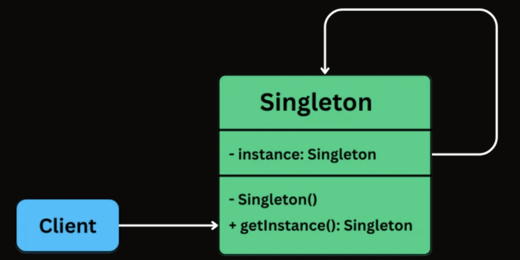
An instance field stores the one and only Singleton object.
The constructor is private or otherwise restricted, so other code cannot create new instances directly.
A getInstance() (or similar) class-level method returns the shared instance and is accessible from anywhere.

🛠 Implementation

class Singleton {
    // Holds the single shared instance (initially not created)
    private static Singleton instance;

    // Private constructor prevents creating objects from outside the class
    private Singleton() {}

    // Global access point to get the Singleton instance
    public static Singleton getInstance() {

        // Create the instance only when first requested (initialization)
        if (instance == null) {
            instance = new Singleton();
        }

        // Return the shared instance
        return instance;
    }
}

class Singleton:
    # Holds the single shared instance (initially not created)
    _instance = None

    # Constructor prevents direct creation if instance already exists
    def __init__(self):
        if Singleton._instance is not None:
            raise Exception("Use get_instance() instead.")

    # Global access point to get the Singleton instance
    @staticmethod
    def get_instance():

        # Create the instance only when first requested (lazy initialization)
        if Singleton._instance is None:
            Singleton._instance = Singleton()

        # Return the shared instance
        return Singleton._instance

class Singleton {
private:
    // Holds the single shared instance (initially not created)
    static Singleton* instance;

    // Private constructor prevents creating objects from outside the class
    Singleton() {}

public:

    // Global access point to get the Singleton instance
    static Singleton* getInstance() {

        // Create the instance only when first requested (initialization)
        if (instance == nullptr) {
            instance = new Singleton();
        }

        // Return the shared instance
        return instance;
    }
};

class Singleton
{
    // Holds the single shared instance (initially not created)
    private static Singleton instance;

    // Private constructor prevents creating objects from outside the class
    private Singleton() { }

    // Global access point to get the Singleton instance
    public static Singleton GetInstance()
    {
        // Create the instance only when first requested (initialization)
        if (instance == null)
        {
            instance = new Singleton();
        }

        // Return the shared instance
        return instance;
    }
}

class Singleton {
  // Holds the single shared instance (initially not created)
  private static instance: Singleton;

  // Private constructor prevents creating objects from outside the class
  private constructor() {}

  // Global access point to get the Singleton instance
  public static getInstance(): Singleton {
    // Create the instance only when first requested (initialization)
    if (Singleton.instance == null) {
      Singleton.instance = new Singleton();
    }

    // Return the shared instance
    return Singleton.instance;
  }
}

Factory Method

📖 Definition

The Factory Method Design Pattern is a creational pattern that provides an interface for creating objects in a superclass, but allows subclasses to alter the type of objects that will be created.

It’s particularly useful in situations where:

The exact type of object to be created isn’t known until runtime.
Object creation logic is complex, repetitive, or needs encapsulation.
You want to follow the Open/Closed Principle, open for extension, closed for modification.

🧩 Class Diagram

Factory Method Class Diagram

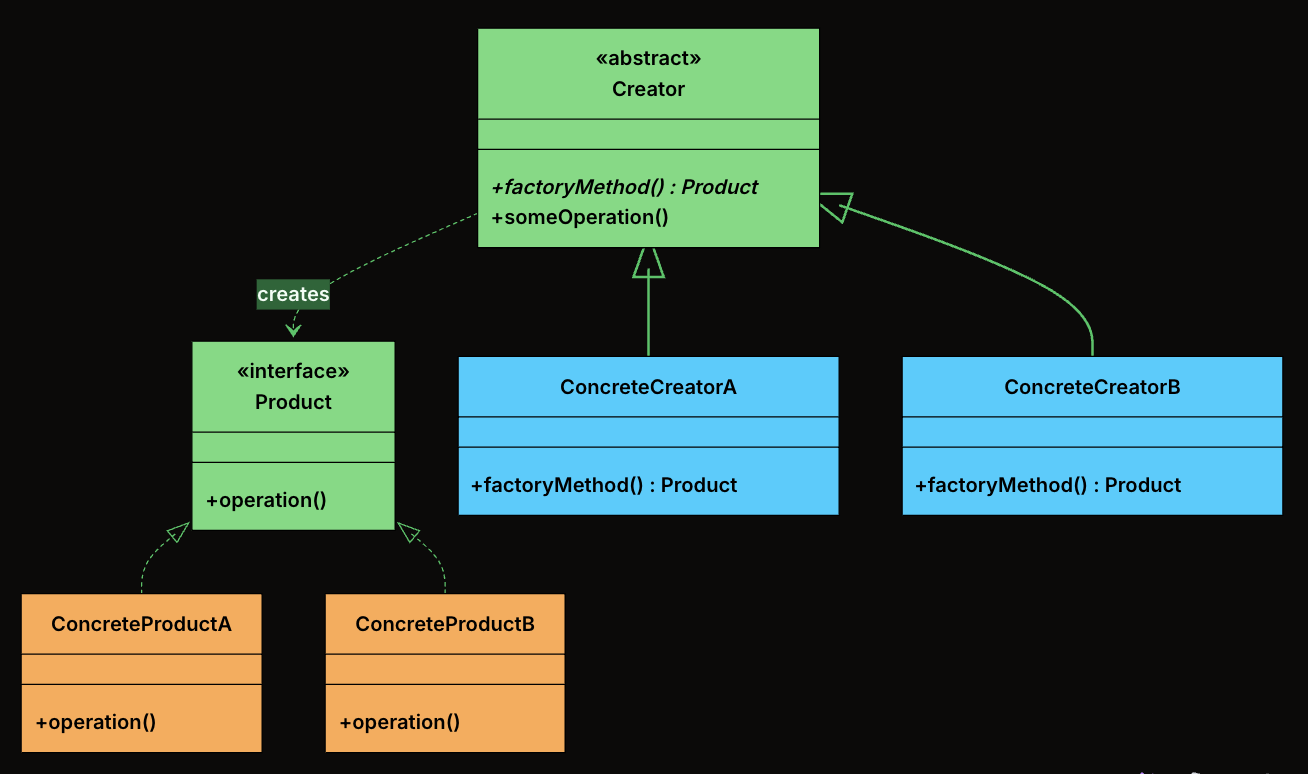
Product: The interface or abstract class that defines the contract for all objects the factory method creates. Every concrete product implements this interface, which means the rest of the system can work with any product without knowing its concrete type.
ConcreteProduct: The actual classes that implement the Product interface. Each one provides its own behavior.
Creator: An abstract class (or an interface) that declares the factory method, which returns an object of type Product.
ConcreteCreator: Subclasses of Creator that override the factory method to return a specific ConcreteProduct. Each creator is paired with exactly one product type.

🛠 Implementation

Define the Product Interface

interface Notification {
    public void send(String message);
}

Define Concrete Products

class EmailNotification implements Notification {
    @Override
    public void send(String message) {
        System.out.println("Sending email: " + message);
    }
}

class SMSNotification implements Notification {
    @Override
    public void send(String message) {
        System.out.println("Sending SMS: " + message);
    }
}

class PushNotification implements Notification {
    @Override
    public void send(String message) {
        System.out.println("Sending push notification: " + message);
    }
}

class SlackNotification implements Notification {
    @Override
    public void send(String message) {
        System.out.println("Sending Slack message: " + message);
    }
}

Define Abstract Creator

abstract class NotificationCreator {
    // Factory Method - subclasses decide what to create
    public abstract Notification createNotification();

    // Shared logic that uses the factory method
    public void send(String message) {
        Notification notification = createNotification();
        notification.send(message);
    }
}

Define Concrete Creators

class EmailNotificationCreator extends NotificationCreator {
    @Override
    public Notification createNotification() {
        return new EmailNotification();
    }
}

class SMSNotificationCreator extends NotificationCreator {
    @Override
    public Notification createNotification() {
        return new SMSNotification();
    }
}

class PushNotificationCreator extends NotificationCreator {
    @Override
    public Notification createNotification() {
        return new PushNotification();
    }
}

class SlackNotificationCreator extends NotificationCreator {
    @Override
    public Notification createNotification() {
        return new SlackNotification();
    }
}

Client Code

public class FactoryMethodDemo {
    public static void main(String[] args) {
        NotificationCreator creator;

        // Send Email
        creator = new EmailNotificationCreator();
        creator.send("Welcome to our platform!");

        // Send SMS
        creator = new SMSNotificationCreator();
        creator.send("Your OTP is 123456");

        // Send Push Notification
        creator = new PushNotificationCreator();
        creator.send("You have a new follower!");

        // Send Slack Message
        creator = new SlackNotificationCreator();
        creator.send("Standup in 10 minutes!");
    }
}

Define the Product Interface

from abc import ABC, abstractmethod

class Notification(ABC):
    @abstractmethod
    def send(self, message: str) -> None:
        pass

Define Concrete Products

class EmailNotification(Notification):
    def send(self, message: str) -> None:
        print(f"Sending email: {message}")

class SMSNotification(Notification):
    def send(self, message: str) -> None:
        print(f"Sending SMS: {message}")

class PushNotification(Notification):
    def send(self, message: str) -> None:
        print(f"Sending push notification: {message}")

class SlackNotification(Notification):
    def send(self, message: str) -> None:
        print(f"Sending Slack message: {message}")

Define Abstract Creator

class NotificationCreator(ABC):
    # Factory Method - subclasses decide what to create
    @abstractmethod
    def create_notification(self) -> Notification:
        pass

    # Shared logic that uses the factory method
    def send(self, message: str) -> None:
        notification = self.create_notification()
        notification.send(message)

Define Concrete Creators

class EmailNotificationCreator(NotificationCreator):
    def create_notification(self) -> Notification:
        return EmailNotification()

class SMSNotificationCreator(NotificationCreator):
    def create_notification(self) -> Notification:
        return SMSNotification()

class PushNotificationCreator(NotificationCreator):
    def create_notification(self) -> Notification:
        return PushNotification()

class SlackNotificationCreator(NotificationCreator):
    def create_notification(self) -> Notification:
        return SlackNotification()

Client Code

def main():
    # Send Email
    creator = EmailNotificationCreator()
    creator.send("Welcome to our platform!")

    # Send SMS
    creator = SMSNotificationCreator()
    creator.send("Your OTP is 123456")

    # Send Push Notification
    creator = PushNotificationCreator()
    creator.send("You have a new follower!")

    # Send Slack Message
    creator = SlackNotificationCreator()
    creator.send("Standup in 10 minutes!")

if __name__ == "__main__":
    main()

Define the Product Interface

class Notification {
public:
    virtual void send(const string& message) = 0;
    virtual ~Notification() {}
};

Define Concrete Products

class EmailNotification : public Notification {
public:
    void send(const string& message) override {
        cout << "Sending email: " << message << endl;
    }
};

class SMSNotification : public Notification {
public:
    void send(const string& message) override {
        cout << "Sending SMS: " << message << endl;
    }
};

class PushNotification : public Notification {
public:
    void send(const string& message) override {
        cout << "Sending push notification: " << message << endl;
    }
};

class SlackNotification : public Notification {
public:
    void send(const string& message) override {
        cout << "Sending Slack message: " << message << endl;
    }
};

Define Abstract Creator

class NotificationCreator {
public:
    // Factory Method - subclasses decide what to create
    virtual unique_ptr<Notification> createNotification() = 0;

    // Shared logic that uses the factory method
    void send(const string& message) {
        auto notification = createNotification();
        notification->send(message);
    }

    virtual ~NotificationCreator() = default;
};

Define Concrete Creators

class EmailNotificationCreator : public NotificationCreator {
public:
    unique_ptr<Notification> createNotification() override {
        return make_unique<EmailNotification>();
    }
};

class SMSNotificationCreator : public NotificationCreator {
public:
    unique_ptr<Notification> createNotification() override {
        return make_unique<SMSNotification>();
    }
};

class PushNotificationCreator : public NotificationCreator {
public:
    unique_ptr<Notification> createNotification() override {
        return make_unique<PushNotification>();
    }
};

class SlackNotificationCreator : public NotificationCreator {
public:
    unique_ptr<Notification> createNotification() override {
        return make_unique<SlackNotification>();
    }
};

Client Code

int main() {
    // Send Email
    unique_ptr<NotificationCreator> creator = make_unique<EmailNotificationCreator>();
    creator->send("Welcome to our platform!");

    // Send SMS
    creator = make_unique<SMSNotificationCreator>();
    creator->send("Your OTP is 123456");

    // Send Push Notification
    creator = make_unique<PushNotificationCreator>();
    creator->send("You have a new follower!");

    // Send Slack Message
    creator = make_unique<SlackNotificationCreator>();
    creator->send("Standup in 10 minutes!");

    return 0;
}

Define the Product Interface

interface INotification
{
    void Send(string message);
}

Define Concrete Products

class EmailNotification : INotification
{
    public void Send(string message)
    {
        Console.WriteLine("Sending email: " + message);
    }
}

class SmsNotification : INotification
{
    public void Send(string message)
    {
        Console.WriteLine("Sending SMS: " + message);
    }
}

class PushNotification : INotification
{
    public void Send(string message)
    {
        Console.WriteLine("Sending push notification: " + message);
    }
}

class SlackNotification : INotification
{
    public void Send(string message)
    {
        Console.WriteLine("Sending Slack message: " + message);
    }
}

Define Abstract Creator

abstract class NotificationCreator
{
    // Factory Method - subclasses decide what to create
    public abstract INotification CreateNotification();

    // Shared logic that uses the factory method
    public void Send(string message)
    {
        INotification notification = CreateNotification();
        notification.Send(message);
    }
}

Define Concrete Creators

class EmailNotificationCreator : NotificationCreator
{
    public override INotification CreateNotification()
    {
        return new EmailNotification();
    }
}

class SmsNotificationCreator : NotificationCreator
{
    public override INotification CreateNotification()
    {
        return new SmsNotification();
    }
}

class PushNotificationCreator : NotificationCreator
{
    public override INotification CreateNotification()
    {
        return new PushNotification();
    }
}

class SlackNotificationCreator : NotificationCreator
{
    public override INotification CreateNotification()
    {
        return new SlackNotification();
    }
}

Client Code

class Program
{
    static void Main()
    {
        NotificationCreator creator;

        // Send Email
        creator = new EmailNotificationCreator();
        creator.Send("Welcome to our platform!");

        // Send SMS
        creator = new SmsNotificationCreator();
        creator.Send("Your OTP is 123456");

        // Send Push Notification
        creator = new PushNotificationCreator();
        creator.Send("You have a new follower!");

        // Send Slack Message
        creator = new SlackNotificationCreator();
        creator.Send("Standup in 10 minutes!");
    }
}

Define the Product Interface

interface Notification {
  send(message: string): void;
}

Define Concrete Products

class EmailNotification implements Notification {
  send(message: string): void {
    console.log(`Sending email: ${message}`);
  }
}

class SMSNotification implements Notification {
  send(message: string): void {
    console.log(`Sending SMS: ${message}`);
  }
}

class PushNotification implements Notification {
  send(message: string): void {
    console.log(`Sending push notification: ${message}`);
  }
}

class SlackNotification implements Notification {
  send(message: string): void {
    console.log(`Sending Slack message: ${message}`);
  }
}

Define Abstract Creator

abstract class NotificationCreator {
  // Factory Method - subclasses decide what to create
  abstract createNotification(): Notification;

  // Shared logic that uses the factory method
  send(message: string): void {
    const notification = this.createNotification();
    notification.send(message);
  }
}

Define Concrete Creators

class EmailNotificationCreator extends NotificationCreator {
  createNotification(): Notification {
    return new EmailNotification();
  }
}

class SMSNotificationCreator extends NotificationCreator {
  createNotification(): Notification {
    return new SMSNotification();
  }
}

class PushNotificationCreator extends NotificationCreator {
  createNotification(): Notification {
    return new PushNotification();
  }
}

class SlackNotificationCreator extends NotificationCreator {
  createNotification(): Notification {
    return new SlackNotification();
  }
}

Client Code

function main(): void {
  let creator: NotificationCreator;

  // Send Email
  creator = new EmailNotificationCreator();
  creator.send("Welcome to our platform!");

  // Send SMS
  creator = new SMSNotificationCreator();
  creator.send("Your OTP is 123456");

  // Send Push Notification
  creator = new PushNotificationCreator();
  creator.send("You have a new follower!");

  // Send Slack Message
  creator = new SlackNotificationCreator();
  creator.send("Standup in 10 minutes!");
}

main();

Abstract Factory

📖 Definition

The Abstract Factory Design Pattern is a creational pattern that provides an interface for creating families of related or dependent objects without specifying their concrete classes.

It’s particularly useful in situations where:

You need to create objects that must be used together and are part of a consistent family (e.g., GUI elements like buttons, checkboxes, and menus).
Your system must support multiple configurations, environments, or product variants (e.g., light vs. dark themes, Windows vs. macOS look-and-feel).
You want to enforce consistency across related objects, ensuring that they are all created from the same factory.

🧩 Class Diagram

Abstract Factory Class Diagram

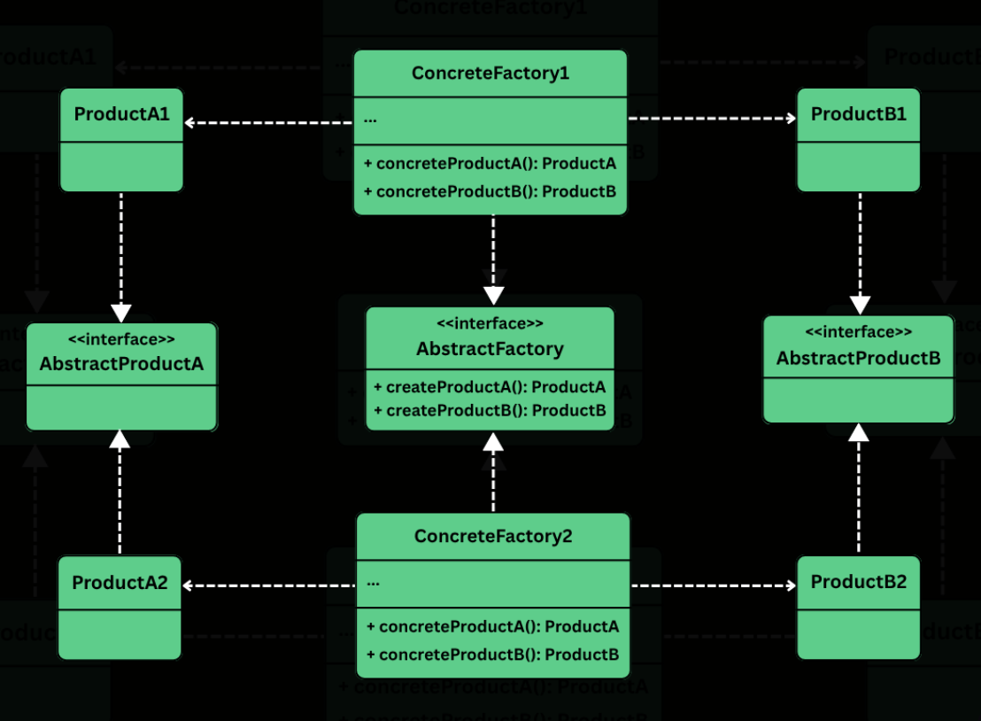
Abstract Factory
- Defines a common interface for creating a family of related products.
- Typically includes factory methods like createButton(), createCheckbox(), createTextField(), etc.
- Clients rely on this interface to create objects without knowing their concrete types.
Concrete Factory
- Implement the abstract factory interface.
- Create concrete product variants that belong to a specific family or platform.
- Each factory ensures that all components it produces are compatible (i.e., belong to the same platform/theme).
Abstract Product
- Define the interfaces or abstract classes for a set of related components.
- All product variants for a given type (e.g., WindowsButton, MacOSButton) will implement these interfaces.
Concrete Product
- Implement the abstract product interfaces.
- Contain platform-specific logic and appearance for the components.
Client
- Uses the abstract factory and abstract product interfaces.
- Is completely unaware of the concrete classes it is using — it only interacts with the factory and product interfaces.
- Can switch entire product families (e.g., from Windows to macOS) by changing the factory without touching UI logic.

🛠 Implementation

Define Abstract Product Interfaces

Button

interface Button {
    void paint();
    void onClick();
}

Checkbox

interface Checkbox {
    void paint();
    void onSelect();
}

Create Concrete Products

Windows Products

class WindowsButton implements Button {
    @Override
    public void paint() {
        System.out.println("Painting a Windows-style button.");
    }

    @Override
    public void onClick() {
        System.out.println("Windows button clicked.");
    }
}

class WindowsCheckbox implements Checkbox {
    @Override
    public void paint() {
        System.out.println("Painting a Windows-style checkbox.");
    }

    @Override
    public void onSelect() {
        System.out.println("Windows checkbox selected.");
    }
}

MacOS Products

class MacOSButton implements Button {
    @Override
    public void paint() {
        System.out.println("Painting a macOS-style button.");
    }

    @Override
    public void onClick() {
        System.out.println("macOS button clicked.");
    }
}

class MacOSCheckbox implements Checkbox {
    @Override
    public void paint() {
        System.out.println("Painting a macOS-style checkbox.");
    }

    @Override
    public void onSelect() {
        System.out.println("macOS checkbox selected.");
    }
}

Define the Abstract Factory

interface GUIFactory {
    Button createButton();
    Checkbox createCheckbox();
}

Implement Concrete Factories

WindowsFactory

class WindowsFactory implements GUIFactory {
    @Override
    public Button createButton() {
        return new WindowsButton();
    }

    @Override
    public Checkbox createCheckbox() {
        return new WindowsCheckbox();
    }
}

MacOSFactory

class MacOSFactory implements GUIFactory {
    @Override
    public Button createButton() {
        return new MacOSButton();
    }

    @Override
    public Checkbox createCheckbox() {
        return new MacOSCheckbox();
    }
}

Client Code

class Application {
    private final Button button;
    private final Checkbox checkbox;

    public Application(GUIFactory factory) {
        this.button = factory.createButton();
        this.checkbox = factory.createCheckbox();
    }

    public void renderUI() {
        button.paint();
        checkbox.paint();
    }
}

Wire Everything Together

public class AppLauncher {
    public static void main(String[] args) {
        // Simulate platform detection
        String os = System.getProperty("os.name");
        GUIFactory factory;

        if (os.contains("Windows")) {
            factory = new WindowsFactory();
        } else {
            factory = new MacOSFactory();
        }

        Application app = new Application(factory);
        app.renderUI();
    }
}

Output (on MacOS)

Painting a macOS-style button.
Painting a macOS-style checkbox.

Output (on Windows)

Painting a Windows-style button.
Painting a Windows-style checkbox.

Define Abstract Product Interfaces

Button

from abc import ABC, abstractmethod

class Button(ABC):
    @abstractmethod
    def paint(self):
        pass

    @abstractmethod
    def on_click(self):
        pass

Checkbox

class Checkbox(ABC):
    @abstractmethod
    def paint(self):
        pass

    @abstractmethod
    def on_select(self):
        pass

Create Concrete Products

Windows Products

class WindowsButton(Button):
    def paint(self):
        print("Painting a Windows-style button.")

    def on_click(self):
        print("Windows button clicked.")


class WindowsCheckbox(Checkbox):
    def paint(self):
        print("Painting a Windows-style checkbox.")

    def on_select(self):
        print("Windows checkbox selected.")

MacOS Products

class MacOSButton(Button):
    def paint(self):
        print("Painting a macOS-style button.")

    def on_click(self):
        print("macOS button clicked.")


class MacOSCheckbox(Checkbox):
    def paint(self):
        print("Painting a macOS-style checkbox.")

    def on_select(self):
        print("macOS checkbox selected.")

Define the Abstract Factory

class GUIFactory(ABC):
    @abstractmethod
    def create_button(self):
        pass

    @abstractmethod
    def create_checkbox(self):
        pass

Implement Concrete Factories

WindowsFactory

class WindowsFactory(GUIFactory):
    def create_button(self):
        return WindowsButton()

    def create_checkbox(self):
        return WindowsCheckbox()

MacOSFactory

class MacOSFactory(GUIFactory):
    def create_button(self):
        return MacOSButton()

    def create_checkbox(self):
        return MacOSCheckbox()

Client Code

class Application:
    def __init__(self, factory):
        self.button = factory.create_button()
        self.checkbox = factory.create_checkbox()

    def render_ui(self):
        self.button.paint()
        self.checkbox.paint()

Wire Everything Together

import platform

class AppLauncher:
    @staticmethod
    def main():
        # Simulate platform detection
        os = platform.system()

        if "Windows" in os:
            factory = WindowsFactory()
        else:
            factory = MacOSFactory()

        app = Application(factory)
        app.render_ui()

if __name__ == "__main__":
    AppLauncher.main()

Output (on MacOS)

Painting a macOS-style button.
Painting a macOS-style checkbox.

Output (on Windows)

Painting a Windows-style button.
Painting a Windows-style checkbox.

Define Abstract Product Interfaces

Button

class Button {
public:
    virtual void paint() = 0;
    virtual void onClick() = 0;
    virtual ~Button() = default;
};

Checkbox

class Checkbox {
public:
    virtual void paint() = 0;
    virtual void onSelect() = 0;
    virtual ~Checkbox() {}
};

Create Concrete Products

Windows Products

class WindowsButton : public Button {
public:
    void paint() override {
        cout << "Painting a Windows-style button." << endl;
    }

    void onClick() override {
        cout << "Windows button clicked." << endl;
    }
};

class WindowsCheckbox : public Checkbox {
public:
    void paint() override {
        cout << "Painting a Windows-style checkbox." << endl;
    }

    void onSelect() override {
        cout << "Windows checkbox selected." << endl;
    }
};

MacOS Products

class MacOSButton : public Button {
public:
    void paint() override {
        cout << "Painting a macOS-style button." << endl;
    }

    void onClick() override {
        cout << "macOS button clicked." << endl;
    }
};

class MacOSCheckbox : public Checkbox {
public:
    void paint() override {
        cout << "Painting a macOS-style checkbox." << endl;
    }

    void onSelect() override {
        cout << "macOS checkbox selected." << endl;
    }
};

Define the Abstract Factory

class GUIFactory {
public:
    virtual Button* createButton() = 0;
    virtual Checkbox* createCheckbox() = 0;
    virtual ~GUIFactory() {}
};

Implement Concrete Factories

WindowsFactory

class WindowsFactory : public GUIFactory {
public:
    Button* createButton() override {
        return new WindowsButton();
    }
    Checkbox* createCheckbox() override {
        return new WindowsCheckbox();
    }
};

MacOSFactory

class MacOSFactory : public GUIFactory {
public:
    Button* createButton() override {
        return new MacOSButton();
    }
    Checkbox* createCheckbox() override {
        return new MacOSCheckbox();
    }
};

Client Code

class Application {
private:
    Button* button;
    Checkbox* checkbox;

public:
    Application(GUIFactory* factory) {
        button = factory->createButton();
        checkbox = factory->createCheckbox();
    }

    ~Application() {
        delete button;
        delete checkbox;
    }

    void renderUI() {
        button->paint();
        checkbox->paint();
    }
};

Wire Everything Together

int main() {
    string os;
    cout << "Enter OS (Windows/Mac): ";
    getline(cin, os);

    GUIFactory* factory = nullptr;

    // Simulated platform detection
    transform(os.begin(), os.end(), os.begin(), ::tolower);
    if (os.find("windows") != string::npos) {
        factory = new WindowsFactory();
    } else {
        factory = new MacOSFactory();
    }

    Application app(factory);
    app.renderUI();

    delete factory;

    return 0;
}

Output (on MacOS)

Painting a macOS-style button.
Painting a macOS-style checkbox.

Output (on Windows)

Painting a Windows-style button.
Painting a Windows-style checkbox.

Define Abstract Product Interfaces

Button

interface IButton
{
    void Paint();
    void OnClick();
}

Checkbox

interface ICheckbox
{
    void Paint();
    void OnSelect();
}

Create Concrete Products

Windows Products

class WindowsButton : IButton
{
    public void Paint()
    {
        Console.WriteLine("Painting a Windows-style button.");
    }

    public void OnClick()
    {
        Console.WriteLine("Windows button clicked.");
    }
}

class WindowsCheckbox : ICheckbox
{
    public void Paint()
    {
        Console.WriteLine("Painting a Windows-style checkbox.");
    }

    public void OnSelect()
    {
        Console.WriteLine("Windows checkbox selected.");
    }
}

MacOS Products

class MacOSButton : IButton
{
    public void Paint()
    {
        Console.WriteLine("Painting a macOS-style button.");
    }

    public void OnClick()
    {
        Console.WriteLine("macOS button clicked.");
    }
}

class MacOSCheckbox : ICheckbox
{
    public void Paint()
    {
        Console.WriteLine("Painting a macOS-style checkbox.");
    }

    public void OnSelect()
    {
        Console.WriteLine("macOS checkbox selected.");
    }
}

Define the Abstract Factory

interface IGUIFactory
{
    IButton CreateButton();
    ICheckbox CreateCheckbox();
}

Implement Concrete Factories

WindowsFactory

class WindowsFactory : IGUIFactory
{
    public IButton CreateButton()
    {
        return new WindowsButton();
    }

    public ICheckbox CreateCheckbox()
    {
        return new WindowsCheckbox();
    }
}

MacOSFactory

class MacOSFactory : IGUIFactory
{
    public IButton CreateButton()
    {
        return new MacOSButton();
    }

    public ICheckbox CreateCheckbox()
    {
        return new MacOSCheckbox();
    }
}

Client Code

class Application
{
    private readonly IButton _button;
    private readonly ICheckbox _checkbox;

    public Application(IGUIFactory factory)
    {
        _button = factory.CreateButton();
        _checkbox = factory.CreateCheckbox();
    }

    public void RenderUI()
    {
        _button.Paint();
        _checkbox.Paint();
    }
}

Wire Everything Together

public class AppLauncher
{
    public static void Main()
    {
        Console.Write("Enter OS (Windows/Mac): ");
        string os = Console.ReadLine()?.ToLower() ?? "";

        IGUIFactory factory;

        if (os.Contains("windows"))
        {
            factory = new WindowsFactory();
        }
        else
        {
            factory = new MacOSFactory();
        }

        Application app = new Application(factory);
        app.RenderUI();
    }
}

Output (on MacOS)

Painting a macOS-style button.
Painting a macOS-style checkbox.

Output (on Windows)

Painting a Windows-style button.
Painting a Windows-style checkbox.

Define Abstract Product Interfaces

Button

interface Button {
  paint(): void;
  onClick(): void;
}

Checkbox

interface Checkbox {
  paint(): void;
  onSelect(): void;
}

Create Concrete Products

Windows Products

class WindowsButton implements Button {
  paint(): void {
    console.log("Painting a Windows-style button.");
  }

  onClick(): void {
    console.log("Windows button clicked.");
  }
}

class WindowsCheckbox implements Checkbox {
  paint(): void {
    console.log("Painting a Windows-style checkbox.");
  }

  onSelect(): void {
    console.log("Windows checkbox selected.");
  }
}

MacOS Products

class MacOSButton implements Button {
  paint(): void {
    console.log("Painting a macOS-style button.");
  }

  onClick(): void {
    console.log("macOS button clicked.");
  }
}

class MacOSCheckbox implements Checkbox {
  paint(): void {
    console.log("Painting a macOS-style checkbox.");
  }

  onSelect(): void {
    console.log("macOS checkbox selected.");
  }
}

Define the Abstract Factory

interface GUIFactory {
  createButton(): Button;
  createCheckbox(): Checkbox;
}

Implement Concrete Factories

WindowsFactory

class WindowsFactory implements GUIFactory {
  createButton(): Button {
    return new WindowsButton();
  }

  createCheckbox(): Checkbox {
    return new WindowsCheckbox();
  }
}

MacOSFactory

class MacOSFactory implements GUIFactory {
  createButton(): Button {
    return new MacOSButton();
  }

  createCheckbox(): Checkbox {
    return new MacOSCheckbox();
  }
}

Client Code

class Application {
  private readonly button: Button;
  private readonly checkbox: Checkbox;

  constructor(factory: GUIFactory) {
    this.button = factory.createButton();
    this.checkbox = factory.createCheckbox();
  }

  renderUI(): void {
    this.button.paint();
    this.checkbox.paint();
  }
}

Wire Everything Together

class AppLauncher {
  static main(): void {
    // Simulate platform detection
    const os = process.platform;
    let factory: GUIFactory;

    if (os === "win32") {
      factory = new WindowsFactory();
    } else {
      factory = new MacOSFactory();
    }

    const app = new Application(factory);
    app.renderUI();
  }
}

AppLauncher.main();

Output (on MacOS)

Painting a macOS-style button.
Painting a macOS-style checkbox.

Output (on Windows)

Painting a Windows-style button.
Painting a Windows-style checkbox.

Builder

📖 Definition

The Builder Design Pattern is a creational pattern that lets you construct complex objects step-by-step, separating the construction logic from the final representation.

Two ideas define the pattern:

Step-by-step construction: Instead of passing everything to a constructor at once, you set each field through individual method calls. You only call the methods for the fields you need.
Fluent interface: Each setter method returns the builder itself, allowing you to chain calls into a single readable expression that ends with build().

🧩 Class Diagram

The Builder pattern involves four participants. In many real-world implementations, the Director is optional and is often skipped when using fluent builders.

Builder Class Diagram

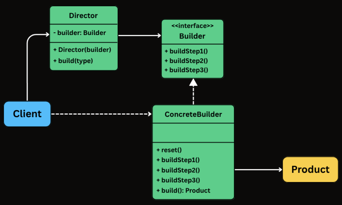
Builder
- Exposes methods to configure the product step by step.
- Typically returns the builder itself from each method to enable fluent chaining.
- Often implemented as a static nested class inside the product class.
ConcreteBuilder
- Implements the builder API (either via an interface or directly through fluent methods).
- Stores intermediate state for the object being constructed.
- Implements build() to validate inputs and produce the final product instance.
Product
- The complex object being constructed.
- Often immutable and created only through the builder.
- Commonly has a private constructor that copies state from the builder.
Director (Optional)
- Coordinates the construction process by calling builder steps in a specific sequence.
- Useful when you want to encapsulate standard configurations or reusable construction sequences.
- Often omitted in fluent builder style, where the client effectively plays this role by chaining builder calls.

🛠 Implementation

Create the Product and Builder

class HttpRequest {
    // Required
    private final String url;

    // Optional
    private final String method;
    private final Map<String, String> headers;
    private final Map<String, String> queryParams;
    private final String body;
    private final int timeout;

    // Private constructor - only the Builder can call this
    private HttpRequest(Builder builder) {
        this.url = builder.url;
        this.method = builder.method;
        this.headers = Collections.unmodifiableMap(new HashMap<>(builder.headers));
        this.queryParams = Collections.unmodifiableMap(new HashMap<>(builder.queryParams));
        this.body = builder.body;
        this.timeout = builder.timeout;
    }

    public String getUrl() { return url; }
    public String getMethod() { return method; }
    public Map<String, String> getHeaders() { return headers; }
    public Map<String, String> getQueryParams() { return queryParams; }
    public String getBody() { return body; }
    public int getTimeout() { return timeout; }

    @Override
    public String toString() {
        return "HttpRequest{url='" + url + "', method='" + method +
               "', headers=" + headers + ", queryParams=" + queryParams +
               ", body='" + body + "', timeout=" + timeout + "}";
    }

    // Static nested Builder class
    public static class Builder {
        private final String url; // required
        private String method = "GET";
        private Map<String, String> headers = new HashMap<>();
        private Map<String, String> queryParams = new HashMap<>();
        private String body;
        private int timeout = 30000;

        public Builder(String url) {
            this.url = url;
        }

        public Builder method(String method) {
            this.method = method;
            return this;
        }

        public Builder addHeader(String key, String value) {
            this.headers.put(key, value);
            return this;
        }

        public Builder addQueryParam(String key, String value) {
            this.queryParams.put(key, value);
            return this;
        }

        public Builder body(String body) {
            this.body = body;
            return this;
        }

        public Builder timeout(int timeout) {
            this.timeout = timeout;
            return this;
        }

        public HttpRequest build() {
            return new HttpRequest(this);
        }
    }
}

Using the Builder from Client Code

public class Main {
    public static void main(String[] args) {
        // Simple GET request - just the URL
        HttpRequest get = new HttpRequest.Builder("https://api.example.com/users")
                .build();

        // POST with body and custom timeout
        HttpRequest post = new HttpRequest.Builder("https://api.example.com/users")
                .method("POST")
                .addHeader("Content-Type", "application/json")
                .body("{\"name\":\"Alice\",\"email\":\"alice@example.com\"}")
                .timeout(5000)
                .build();

        // Authenticated PUT with query parameters
        HttpRequest put = new HttpRequest.Builder("https://api.example.com/config")
                .method("PUT")
                .addHeader("Authorization", "Bearer token123")
                .addHeader("Content-Type", "application/json")
                .addQueryParam("env", "production")
                .addQueryParam("version", "2")
                .body("{\"feature_flag\":true}")
                .timeout(10000)
                .build();
    }
}

Create the Product and Builder

class HttpRequest:
    def __init__(self, builder):
        self.url = builder._url
        self.method = builder._method
        self.headers = dict(builder._headers)  # defensive copy
        self.query_params = dict(builder._query_params)
        self.body = builder._body
        self.timeout = builder._timeout

    def __str__(self):
        return (f"HttpRequest(url='{self.url}', method='{self.method}', "
                f"headers={self.headers}, query_params={self.query_params}, "
                f"body='{self.body}', timeout={self.timeout})")

    class Builder:
        def __init__(self, url):
            self._url = url  # required
            self._method = "GET"
            self._headers = {}
            self._query_params = {}
            self._body = None
            self._timeout = 30000

        def method(self, method):
            self._method = method
            return self

        def add_header(self, key, value):
            self._headers[key] = value
            return self

        def add_query_param(self, key, value):
            self._query_params[key] = value
            return self

        def body(self, body):
            self._body = body
            return self

        def timeout(self, timeout):
            self._timeout = timeout
            return self

        def build(self):
            return HttpRequest(self)

Using the Builder from Client Code

if __name__ == "__main__":
    # Simple GET request
    get = HttpRequest.Builder("https://api.example.com/users") \
        .build()

    # POST with body and custom timeout
    post = HttpRequest.Builder("https://api.example.com/users") \
        .method("POST") \
        .add_header("Content-Type", "application/json") \
        .body('{"name":"Alice","email":"alice@example.com"}') \
        .timeout(5000) \
        .build()

    # Authenticated PUT with query parameters
    put = HttpRequest.Builder("https://api.example.com/config") \
        .method("PUT") \
        .add_header("Authorization", "Bearer token123") \
        .add_header("Content-Type", "application/json") \
        .add_query_param("env", "production") \
        .add_query_param("version", "2") \
        .body('{"feature_flag":true}') \
        .timeout(10000) \
        .build()

Create the Product and Builder

class HttpRequest {
private:
    string url;
    string method;
    map<string, string> headers;
    map<string, string> queryParams;
    string body;
    int timeout;

    // Private constructor
    HttpRequest(const string& url, const string& method,
                const map<string, string>& headers,
                const map<string, string>& queryParams,
                const string& body, int timeout)
        : url(url), method(method), headers(headers),
          queryParams(queryParams), body(body), timeout(timeout) {}

public:
    string getUrl() const {
        return url;
    }
    string getMethod() const {
        return method;
    }

    void print() const {
        cout << "HttpRequest{url='" << url << "', method='" << method
             << "', headers=" << headers.size()
             << ", queryParams=" << queryParams.size()
             << ", body='" << body << "', timeout=" << timeout << "}" << endl;
    }

    class Builder {
    private:
        string url;
        string method = "GET";
        map<string, string> headers;
        map<string, string> queryParams;
        string body;
        int timeout = 30000;

    public:
        explicit Builder(const string& url) : url(url) {}

        Builder& setMethod(const string& m) {
            method = m;
            return *this;
        }

        Builder& addHeader(const string& key, const string& value) {
            headers[key] = value;
            return *this;
        }

        Builder& addQueryParam(const string& key, const string& value) {
            queryParams[key] = value;
            return *this;
        }

        Builder& setBody(const string& b) {
            body = b;
            return *this;
        }

        Builder& setTimeout(int t) {
            timeout = t;
            return *this;
        }

        HttpRequest build() const {
            return HttpRequest(url, method, headers, queryParams, body, timeout);
        }
    };
};

Using the Builder from Client Code

int main() {
    // Simple GET request
    HttpRequest get = HttpRequest::Builder("https://api.example.com/users")
        .build();

    // POST with body and custom timeout
    HttpRequest post = HttpRequest::Builder("https://api.example.com/users")
        .setMethod("POST")
        .addHeader("Content-Type", "application/json")
        .setBody("{\"name\":\"Alice\",\"email\":\"alice@example.com\"}")
        .setTimeout(5000)
        .build();

    // Authenticated PUT with query parameters
    HttpRequest put = HttpRequest::Builder("https://api.example.com/config")
        .setMethod("PUT")
        .addHeader("Authorization", "Bearer token123")
        .addHeader("Content-Type", "application/json")
        .addQueryParam("env", "production")
        .addQueryParam("version", "2")
        .setBody("{\"feature_flag\":true}")
        .setTimeout(10000)
        .build();

    return 0;
}

Create the Product and Builder

class HttpRequest
{
    public string Url { get; }
    public string Method { get; }
    public IReadOnlyDictionary<string, string> Headers { get; }
    public IReadOnlyDictionary<string, string> QueryParams { get; }
    public string Body { get; }
    public int Timeout { get; }

    // Private constructor
    private HttpRequest(Builder builder)
    {
        Url = builder.Url;
        Method = builder.Method;
        Headers = new Dictionary<string, string>(builder.Headers);
        QueryParams = new Dictionary<string, string>(builder.QueryParams);
        Body = builder.Body;
        Timeout = builder.Timeout;
    }

    public override string ToString()
    {
        return $"HttpRequest{{Url='{Url}', Method='{Method}', " +
               $"Headers={Headers.Count}, QueryParams={QueryParams.Count}, " +
               $"Body='{Body}', Timeout={Timeout}}}";
    }

    public class Builder
    {
        public string Url { get; }
        public string Method { get; private set; } = "GET";
        public Dictionary<string, string> Headers { get; } = new();
        public Dictionary<string, string> QueryParams { get; } = new();
        public string Body { get; private set; }
        public int Timeout { get; private set; } = 30000;

        public Builder(string url) {
            Url = url;
        }

        public Builder SetMethod(string method)
        {
            Method = method;
            return this;
        }

        public Builder AddHeader(string key, string value)
        {
            Headers[key] = value;
            return this;
        }

        public Builder AddQueryParam(string key, string value)
        {
            QueryParams[key] = value;
            return this;
        }

        public Builder SetBody(string body)
        {
            Body = body;
            return this;
        }

        public Builder SetTimeout(int timeout)
        {
            Timeout = timeout;
            return this;
        }

        public HttpRequest Build()
        {
            return new HttpRequest(this);
        }
    }
}

Using the Builder from Client Code

class Program
{
    static void Main()
    {
        // Simple GET request
        var get = new HttpRequest.Builder("https://api.example.com/users")
            .Build();

        // POST with body and custom timeout
        var post = new HttpRequest.Builder("https://api.example.com/users")
            .SetMethod("POST")
            .AddHeader("Content-Type", "application/json")
            .SetBody("{\"name\":\"Alice\",\"email\":\"alice@example.com\"}")
            .SetTimeout(5000)
            .Build();

        // Authenticated PUT with query parameters
        var put = new HttpRequest.Builder("https://api.example.com/config")
            .SetMethod("PUT")
            .AddHeader("Authorization", "Bearer token123")
            .AddHeader("Content-Type", "application/json")
            .AddQueryParam("env", "production")
            .AddQueryParam("version", "2")
            .SetBody("{\"feature_flag\":true}")
            .SetTimeout(10000)
            .Build();
    }
}

Create the Product and Builder

class HttpRequest {
  private readonly url: string;
  private readonly method: string;
  private readonly headers: ReadonlyMap<string, string>;
  private readonly queryParams: ReadonlyMap<string, string>;
  private readonly body: string | null;
  private readonly timeout: number;

  // Private constructor
  private constructor(builder: HttpRequestBuilder) {
    this.url = builder.getUrl();
    this.method = builder.getMethod();
    this.headers = new Map(builder.getHeaders());
    this.queryParams = new Map(builder.getQueryParams());
    this.body = builder.getBody();
    this.timeout = builder.getTimeout();
  }

  toString(): string {
    return (
      `HttpRequest{url='${this.url}', method='${this.method}', ` +
      `headers=${this.headers.size}, queryParams=${this.queryParams.size}, ` +
      `body='${this.body}', timeout=${this.timeout}}`
    );
  }

  static Builder = class HttpRequestBuilder {
    private url: string;
    private method: string = "GET";
    private headers: Map<string, string> = new Map();
    private queryParams: Map<string, string> = new Map();
    private body: string | null = null;
    private timeout: number = 30000;

    constructor(url: string) {
      this.url = url;
    }

    getUrl(): string {
      return this.url;
    }
    getMethod(): string {
      return this.method;
    }
    getHeaders(): Map<string, string> {
      return this.headers;
    }
    getQueryParams(): Map<string, string> {
      return this.queryParams;
    }
    getBody(): string | null {
      return this.body;
    }
    getTimeout(): number {
      return this.timeout;
    }

    setMethod(method: string): this {
      this.method = method;
      return this;
    }

    addHeader(key: string, value: string): this {
      this.headers.set(key, value);
      return this;
    }

    addQueryParam(key: string, value: string): this {
      this.queryParams.set(key, value);
      return this;
    }

    setBody(body: string): this {
      this.body = body;
      return this;
    }

    setTimeout(timeout: number): this {
      this.timeout = timeout;
      return this;
    }

    build(): HttpRequest {
      return new HttpRequest(this);
    }
  };
}

Using the Builder from Client Code

// Simple GET request
const get = new HttpRequest.Builder("https://api.example.com/users").build();

// POST with body and custom timeout
const post = new HttpRequest.Builder("https://api.example.com/users")
  .setMethod("POST")
  .addHeader("Content-Type", "application/json")
  .setBody('{"name":"Alice","email":"alice@example.com"}')
  .setTimeout(5000)
  .build();

// Authenticated PUT with query parameters
const put = new HttpRequest.Builder("https://api.example.com/config")
  .setMethod("PUT")
  .addHeader("Authorization", "Bearer token123")
  .addHeader("Content-Type", "application/json")
  .addQueryParam("env", "production")
  .addQueryParam("version", "2")
  .setBody('{"feature_flag":true}')
  .setTimeout(10000)
  .build();

Structural Patterns

Adapter
Bridge
Decorator
Composite
Facade

Adapter

📖 Definition

The Adapter Design Pattern is a structural design pattern that allows incompatible interfaces to work together by converting the interface of one class into another that the client expects.

It’s particularly useful in situations where:

You’re integrating with a legacy system or a third-party library that doesn’t match your current interface.
You want to reuse existing functionality without modifying its source code.
You need to bridge the gap between new and old code, or between systems built with different interface designs.

🧩 Class Diagram

Adapter Pattern Class Diagram

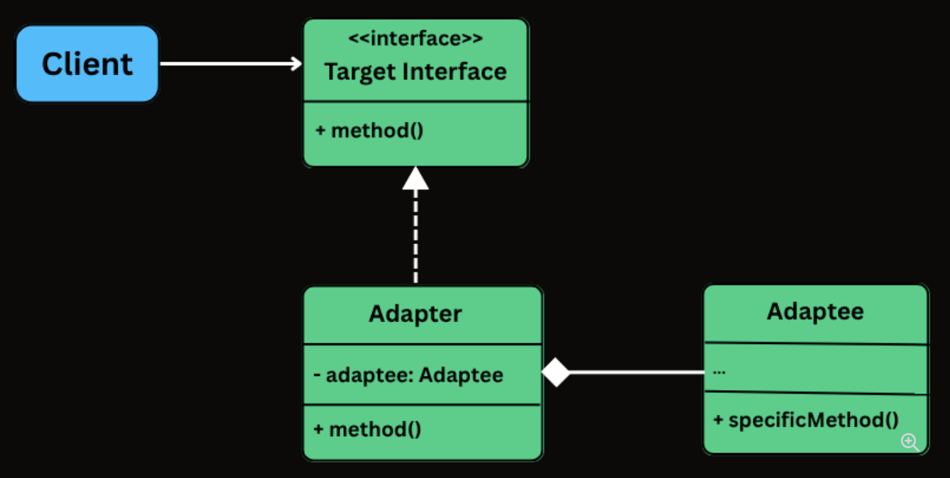
Target Interface: The interface that the client code depends on. Every method call from the client goes through this interface.
Adaptee: The existing class with a useful implementation but an incompatible interface.
Adapter: The translator. It implements the Target interface and holds a reference to the Adaptee, delegating calls with the necessary translation.
Client: The code that uses the Target interface. It is completely unaware of the Adaptee or the Adapter’s internal workings.

🛠 Implementation

Define the Target Interface

interface PaymentProcessor {
    void processPayment(double amount, String currency);
    boolean isPaymentSuccessful();
    String getTransactionId();
}

Create the Adaptee Class

class LegacyGateway {
    private long transactionReference;
    private boolean paymentSuccessful;

    public void executeTransaction(double totalAmount, String currency) {
        System.out.println("LegacyGateway: Executing " + currency + " " + totalAmount);
        transactionReference = System.nanoTime();
        paymentSuccessful = true;
        System.out.println("LegacyGateway: Done. Ref: " + transactionReference);
    }

    public boolean checkStatus(long ref) {
        System.out.println("LegacyGateway: Checking status for ref: " + ref);
        return paymentSuccessful;
    }

    public long getReferenceNumber() {
        return transactionReference;
    }
}

Implement the Adapter Class

class LegacyGatewayAdapter implements PaymentProcessor {
    private final LegacyGateway legacyGateway;
    private long currentRef;

    public LegacyGatewayAdapter(LegacyGateway legacyGateway) {
        this.legacyGateway = legacyGateway;
    }

    @Override
    public void processPayment(double amount, String currency) {
        System.out.println("Adapter: Translating processPayment() for " + amount + " " + currency);
        legacyGateway.executeTransaction(amount, currency);
        currentRef = legacyGateway.getReferenceNumber(); // Store for later use
    }

    @Override
    public boolean isPaymentSuccessful() {
        return legacyGateway.checkStatus(currentRef);
    }

    @Override
    public String getTransactionId() {
        return "LEGACY_TXN_" + currentRef;
    }
}

Client Code

public class ECommerceAppV2 {
    public static void main(String[] args) {
        // Modern processor
        PaymentProcessor processor = new InHousePaymentProcessor();
        CheckoutService modernCheckout = new CheckoutService(processor);
        System.out.println("--- Using Modern Processor ---");
        modernCheckout.checkout(199.99, "USD");

        // Legacy gateway through adapter
        System.out.println("\n--- Using Legacy Gateway via Adapter ---");
        LegacyGateway legacy = new LegacyGateway();
        processor = new LegacyGatewayAdapter(legacy);
        CheckoutService legacyCheckout = new CheckoutService(processor);
        legacyCheckout.checkout(75.50, "USD");
    }
}

Define the Target Interface

from abc import ABC, abstractmethod

class PaymentProcessor(ABC):
    @abstractmethod
    def process_payment(self, amount: float, currency: str):
        pass

    @abstractmethod
    def is_payment_successful(self) -> bool:
        pass

    @abstractmethod
    def get_transaction_id(self) -> str:
        pass

Create the Adaptee Class

class LegacyGateway:
    def __init__(self):
        self._transaction_reference = None
        self._payment_successful = False

    def execute_transaction(self, total_amount: float, currency: str):
        print(f"LegacyGateway: Executing {currency} {total_amount}")
        self._transaction_reference = time.time_ns()
        self._payment_successful = True
        print(f"LegacyGateway: Done. Ref: {self._transaction_reference}")

    def check_status(self, ref: int) -> bool:
        print(f"LegacyGateway: Checking status for ref: {ref}")
        return self._payment_successful

    def get_reference_number(self) -> int:
        return self._transaction_reference

Implement the Adapter Class

class LegacyGatewayAdapter(PaymentProcessor):
   def __init__(self, legacy_gateway):
       self.legacy_gateway = legacy_gateway
       self.current_ref = None

   def process_payment(self, amount, currency):
       print(f"Adapter: Translating processPayment() for {amount} {currency}")
       self.legacy_gateway.execute_transaction(amount, currency)
       self.current_ref = self.legacy_gateway.get_reference_number()

   def is_payment_successful(self):
       return self.legacy_gateway.check_status(self.current_ref)

   def get_transaction_id(self):
       return f"LEGACY_TXN_{self.current_ref}"

Client Code

class ECommerceAppV2:
   @staticmethod
   def main():
       # Modern processor
       processor = InHousePaymentProcessor()
       modern_checkout = CheckoutService(processor)
       print("--- Using Modern Processor ---")
       modern_checkout.checkout(199.99, "USD")

       # Legacy gateway through adapter
       print("\n--- Using Legacy Gateway via Adapter ---")
       legacy = LegacyGateway()
       processor = LegacyGatewayAdapter(legacy)
       legacy_checkout = CheckoutService(processor)
       legacy_checkout.checkout(75.50, "USD")

if __name__ == "__main__":
   ECommerceAppV2.main()

Define the Target Interface

class PaymentProcessor {
public:
   virtual void processPayment(double amount, string currency) = 0;
   virtual bool isPaymentSuccessful() = 0;
   virtual string getTransactionId() = 0;
   virtual ~PaymentProcessor() {}
};

Create the Adaptee Class

class LegacyGateway {
private:
    long transactionReference = 0;
    bool paymentSuccessful = false;

public:
    void executeTransaction(double totalAmount, string currency) {
        cout << "LegacyGateway: Executing " << currency << " " << totalAmount << endl;
        transactionReference = chrono::duration_cast<chrono::nanoseconds>(
            chrono::system_clock::now().time_since_epoch()).count();
        paymentSuccessful = true;
        cout << "LegacyGateway: Done. Ref: " << transactionReference << endl;
    }

    bool checkStatus(long ref) {
        cout << "LegacyGateway: Checking status for ref: " << ref << endl;
        return paymentSuccessful;
    }

    long getReferenceNumber() {
        return transactionReference;
    }
};

Implement the Adapter Class

class LegacyGatewayAdapter : public PaymentProcessor {
private:
   LegacyGateway* legacyGateway;
   long currentRef;

public:
   LegacyGatewayAdapter(LegacyGateway* legacyGateway) : legacyGateway(legacyGateway), currentRef(0) {}

   void processPayment(double amount, string currency) override {
       cout << "Adapter: Translating processPayment() for " << amount << " " << currency << endl;
       legacyGateway->executeTransaction(amount, currency);
       currentRef = legacyGateway->getReferenceNumber();
   }

   bool isPaymentSuccessful() override {
       return legacyGateway->checkStatus(currentRef);
   }

   string getTransactionId() override {
       return "LEGACY_TXN_" + to_string(currentRef);
   }
};

Client Code

class ECommerceAppV2 {
public:
   static void main() {
       // Modern processor
       InHousePaymentProcessor processor;
       CheckoutService modernCheckout(&processor);
       cout << "--- Using Modern Processor ---" << endl;
       modernCheckout.checkout(199.99, "USD");

       // Legacy gateway through adapter
       cout << "\n--- Using Legacy Gateway via Adapter ---" << endl;
       LegacyGateway legacy;
       LegacyGatewayAdapter adapter(&legacy);
       CheckoutService legacyCheckout(&adapter);
       legacyCheckout.checkout(75.50, "USD");
   }
};

int main() {
   ECommerceAppV2::main();
   return 0;
}

Define the Target Interface

interface IPaymentProcessor
{
   void ProcessPayment(double amount, string currency);
   bool IsPaymentSuccessful();
   string GetTransactionId();
}

Create the Adaptee Class

class LegacyGateway
{
    private long transactionReference;
    private bool paymentSuccessful;

    public void ExecuteTransaction(double totalAmount, string currency)
    {
        Console.WriteLine($"LegacyGateway: Executing {currency} {totalAmount}");
        transactionReference = DateTimeOffset.Now.Ticks;
        paymentSuccessful = true;
        Console.WriteLine($"LegacyGateway: Done. Ref: {transactionReference}");
    }

    public bool CheckStatus(long reference)
    {
        Console.WriteLine($"LegacyGateway: Checking status for ref: {reference}");
        return paymentSuccessful;
    }

    public long GetReferenceNumber() => transactionReference;
}

Implement the Adapter Class

class LegacyGatewayAdapter : IPaymentProcessor
{
   private LegacyGateway legacyGateway;
   private long currentRef;

   public LegacyGatewayAdapter(LegacyGateway legacyGateway)
   {
       this.legacyGateway = legacyGateway;
   }

   public void ProcessPayment(double amount, string currency)
   {
       Console.WriteLine($"Adapter: Translating processPayment() for {amount} {currency}");
       legacyGateway.ExecuteTransaction(amount, currency);
       currentRef = legacyGateway.GetReferenceNumber();
   }

   public bool IsPaymentSuccessful()
   {
       return legacyGateway.CheckStatus(currentRef);
   }

   public string GetTransactionId()
   {
       return "LEGACY_TXN_" + currentRef;
   }
}

Client Code

public class ECommerceAppV2
{
   public static void Main(string[] args)
   {
       // Modern processor
       IPaymentProcessor processor = new InHousePaymentProcessor();
       CheckoutService modernCheckout = new CheckoutService(processor);
       Console.WriteLine("--- Using Modern Processor ---");
       modernCheckout.Checkout(199.99, "USD");

       // Legacy gateway through adapter
       Console.WriteLine("\n--- Using Legacy Gateway via Adapter ---");
       LegacyGateway legacy = new LegacyGateway();
       processor = new LegacyGatewayAdapter(legacy);
       CheckoutService legacyCheckout = new CheckoutService(processor);
       legacyCheckout.Checkout(75.50, "USD");
   }
}

Define the Target Interface

interface PaymentProcessor {
  processPayment(amount: number, currency: string): void;
  isPaymentSuccessful(): boolean;
  getTransactionId(): string;
}

Create the Adaptee Class

class LegacyGateway {
  private transactionReference: number = 0;
  private paymentSuccessful: boolean = false;

  executeTransaction(totalAmount: number, currency: string): void {
    console.log(`LegacyGateway: Executing ${currency} ${totalAmount}`);
    this.transactionReference =
      Date.now() * 1000000 + Math.floor(Math.random() * 1000000);
    this.paymentSuccessful = true;
    console.log(`LegacyGateway: Done. Ref: ${this.transactionReference}`);
  }

  checkStatus(ref: number): boolean {
    console.log(`LegacyGateway: Checking status for ref: ${ref}`);
    return this.paymentSuccessful;
  }

  getReferenceNumber(): number {
    return this.transactionReference;
  }
}

Implement the Adapter Class

class LegacyGatewayAdapter implements PaymentProcessor {
  private readonly legacyGateway: LegacyGateway;
  private currentRef: number;

  constructor(legacyGateway: LegacyGateway) {
    this.legacyGateway = legacyGateway;
  }

  processPayment(amount: number, currency: string): void {
    console.log(
      "Adapter: Translating processPayment() for " + amount + " " + currency,
    );
    this.legacyGateway.executeTransaction(amount, currency);
    this.currentRef = this.legacyGateway.getReferenceNumber(); // Store for later use
  }

  isPaymentSuccessful(): boolean {
    return this.legacyGateway.checkStatus(this.currentRef);
  }

  getTransactionId(): string {
    return "LEGACY_TXN_" + this.currentRef;
  }
}

Client Code

class ECommerceAppV2 {
  static main(): void {
    // Modern processor
    let processor: PaymentProcessor = new InHousePaymentProcessor();
    const modernCheckout = new CheckoutService(processor);
    console.log("--- Using Modern Processor ---");
    modernCheckout.checkout(199.99, "USD");

    // Legacy gateway through adapter
    console.log("\n--- Using Legacy Gateway via Adapter ---");
    const legacy = new LegacyGateway();
    processor = new LegacyGatewayAdapter(legacy);
    const legacyCheckout = new CheckoutService(processor);
    legacyCheckout.checkout(75.5, "USD");
  }
}

Bridge

📖 Definition

The Bridge Design Pattern is a structural pattern that lets you decouple an abstraction from its implementation, allowing the two to vary independently.

It’s particularly useful in situations where:

You have classes that can be extended in multiple orthogonal dimensions (e.g., shape vs. rendering technology, UI control vs. platform).
You want to avoid a deep inheritance hierarchy that multiplies combinations of features.
You need to combine multiple variations of behavior or implementation at runtime.

🧩 Class Diagram

Bridge Pattern Class Diagram

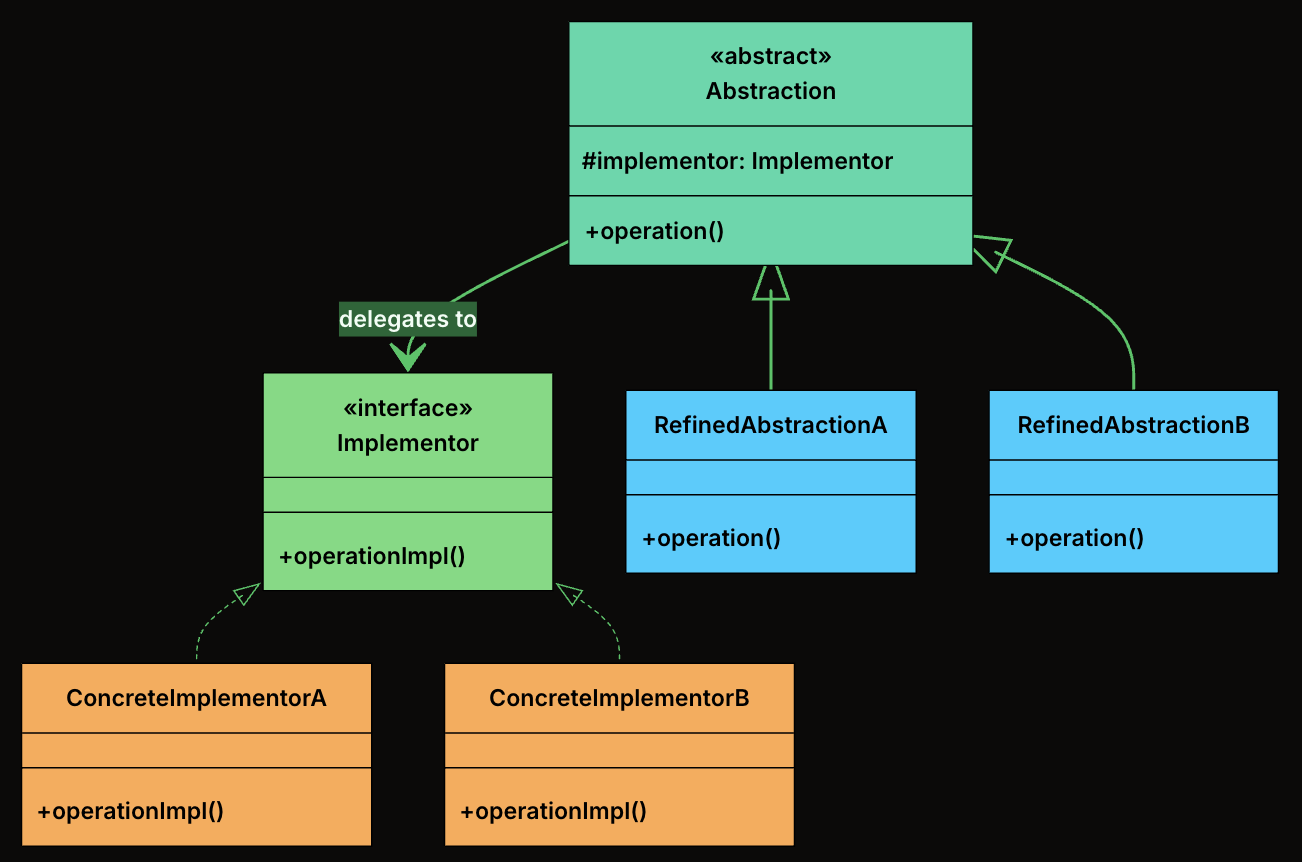
Abstraction: The high-level interface that clients interact with. It defines operations in terms that make sense to the domain (e.g., “draw a shape”) and delegates the low-level work to an implementor.
RefinedAbstraction: A concrete subclass of Abstraction that adds domain-specific state or behavior. It still delegates to the implementor for low-level operations.
Implementor: The interface that defines the low-level operations that concrete implementations must provide. This is the “other side” of the bridge.
ConcreteImplementors: A concrete class that implements the Implementor interface with a specific technology or strategy.

🛠 Implementation

Define Implementator Interface

interface Renderer {
    void renderCircle(float radius);
    void renderRectangle(float width, float height);
}

Create Concrete Implementations of the Renderer

VectorRenderer

class VectorRenderer implements Renderer {
    @Override
    public void renderCircle(float radius) {
        System.out.println("Drawing a circle of radius " + radius + " using VECTOR rendering.");
    }

    @Override
    public void renderRectangle(float width, float height) {
        System.out.println("Drawing a rectangle " + width + "x" + height + " using VECTOR rendering.");
    }
}

RasterRenderer

class RasterRenderer implements Renderer {
    @Override
    public void renderCircle(float radius) {
        System.out.println("Drawing pixels for a circle of radius " + radius + " (RASTER).");
    }

    @Override
    public void renderRectangle(float width, float height) {
        System.out.println("Drawing pixels for a rectangle " + width + "x" + height + " (RASTER).");
    }
}

Define the Abstraction

abstract class Shape {
    protected Renderer renderer;

    public Shape(Renderer renderer) {
        this.renderer = renderer;
    }

    public abstract void draw();
}

Create Concrete Shapes

Circle

class Circle extends Shape {
    private final float radius;

    public Circle(Renderer renderer, float radius) {
        super(renderer);
        this.radius = radius;
    }

    @Override
    public void draw() {
        renderer.renderCircle(radius);
    }
}

Rectangle

class Rectangle extends Shape {
    private final float width;
    private final float height;

    public Rectangle(Renderer renderer, float width, float height) {
        super(renderer);
        this.width = width;
        this.height = height;
    }

    @Override
    public void draw() {
        renderer.renderRectangle(width, height);
    }
}

Client Code

public class BridgeDemo {
    public static void main(String[] args) {
        Renderer vector = new VectorRenderer();
        Renderer raster = new RasterRenderer();

        Shape circle1 = new Circle(vector, 5);
        Shape circle2 = new Circle(raster, 5);

        Shape rectangle1 = new Rectangle(vector, 10, 4);
        Shape rectangle2 = new Rectangle(raster, 10, 4);

        circle1.draw();     // Vector
        circle2.draw();     // Raster
        rectangle1.draw();  // Vector
        rectangle2.draw();  // Raster
    }
}

Define Implementator Interface

from abc import ABC, abstractmethod

class Renderer(ABC):
    @abstractmethod
    def render_circle(self, radius: float):
        pass

    @abstractmethod
    def render_rectangle(self, width: float, height: float):
        pass

Create Concrete Implementations of the Renderer

VectorRenderer

class VectorRenderer(Renderer):
    def render_circle(self, radius):
        print(f"Drawing a circle of radius {radius} using VECTOR rendering.")

    def render_rectangle(self, width, height):
        print(f"Drawing a rectangle {width}x{height} using VECTOR rendering.")

RasterRenderer

class RasterRenderer(Renderer):
    def render_circle(self, radius):
        print(f"Drawing pixels for a circle of radius {radius} (RASTER).")

    def render_rectangle(self, width, height):
        print(f"Drawing pixels for a rectangle {width}x{height} (RASTER).")

Define the Abstraction

class Shape(ABC):
    def __init__(self, renderer):
        self.renderer = renderer

    @abstractmethod
    def draw(self):
        pass

Create Concrete Shapes

Circle

class Circle(Shape):
    def __init__(self, renderer, radius):
        super().__init__(renderer)
        self.radius = radius

    def draw(self):
        self.renderer.render_circle(self.radius)

Rectangle

class Rectangle(Shape):
    def __init__(self, renderer, width, height):
        super().__init__(renderer)
        self.width = width
        self.height = height

    def draw(self):
        self.renderer.render_rectangle(self.width, self.height)

Client Code

def bridge_demo():
    vector = VectorRenderer()
    raster = RasterRenderer()

    circle1 = Circle(vector, 5)
    circle2 = Circle(raster, 5)

    rectangle1 = Rectangle(vector, 10, 4)
    rectangle2 = Rectangle(raster, 10, 4)

    circle1.draw()     # Vector
    circle2.draw()     # Raster
    rectangle1.draw()  # Vector
    rectangle2.draw()  # Raster

# Example usage
if __name__ == "__main__":
    bridge_demo()

Define Implementator Interface

class Renderer {
public:
    virtual ~Renderer() {}
    virtual void renderCircle(float radius) = 0;
    virtual void renderRectangle(float width, float height) = 0;
};

Create Concrete Implementations of the Renderer

VectorRenderer

class VectorRenderer : public Renderer {
public:
    void renderCircle(float radius) override {
        cout << "Drawing a circle of radius " << radius << " using VECTOR rendering." << endl;
    }

    void renderRectangle(float width, float height) override {
        cout << "Drawing a rectangle " << width << "x" << height << " using VECTOR rendering." << endl;
    }
};

RasterRenderer

class RasterRenderer : public Renderer {
public:
    void renderCircle(float radius) override {
        cout << "Drawing pixels for a circle of radius " << radius << " (RASTER)." << endl;
    }

    void renderRectangle(float width, float height) override {
        cout << "Drawing pixels for a rectangle " << width << "x" << height << " (RASTER)." << endl;
    }
};

Define the Abstraction

class Shape {
protected:
    Renderer* renderer;

public:
    Shape(Renderer* renderer) : renderer(renderer) {}
    virtual ~Shape() {}
    virtual void draw() = 0;
};

Create Concrete Shapes

Circle

class Circle : public Shape {
private:
    float radius;

public:
    Circle(Renderer* renderer, float radius) : Shape(renderer), radius(radius) {}

    void draw() override {
        renderer->renderCircle(radius);
    }
};

Rectangle

class Rectangle : public Shape {
private:
    float width;
    float height;

public:
    Rectangle(Renderer* renderer, float width, float height)
        : Shape(renderer), width(width), height(height) {}

    void draw() override {
        renderer->renderRectangle(width, height);
    }
};

Client Code

int main() {
    VectorRenderer vector;
    RasterRenderer raster;

    Circle circle1(&vector, 5);
    Circle circle2(&raster, 5);

    Rectangle rectangle1(&vector, 10, 4);
    Rectangle rectangle2(&raster, 10, 4);

    circle1.draw();     // Vector
    circle2.draw();     // Raster
    rectangle1.draw();  // Vector
    rectangle2.draw();  // Raster

    return 0;
}

Define Implementator Interface

interface IRenderer
{
    void RenderCircle(float radius);
    void RenderRectangle(float width, float height);
}

Create Concrete Implementations of the Renderer

VectorRenderer

class VectorRenderer : IRenderer
{
    public void RenderCircle(float radius)
    {
        Console.WriteLine($"Drawing a circle of radius {radius} using VECTOR rendering.");
    }

    public void RenderRectangle(float width, float height)
    {
        Console.WriteLine($"Drawing a rectangle {width}x{height} using VECTOR rendering.");
    }
}

RasterRenderer

class RasterRenderer : IRenderer
{
    public void RenderCircle(float radius)
    {
        Console.WriteLine($"Drawing pixels for a circle of radius {radius} (RASTER).");
    }

    public void RenderRectangle(float width, float height)
    {
        Console.WriteLine($"Drawing pixels for a rectangle {width}x{height} (RASTER).");
    }
}

Define the Abstraction

abstract class Shape
{
    protected IRenderer renderer;

    public Shape(IRenderer renderer)
    {
        this.renderer = renderer;
    }

    public abstract void Draw();
}

Create Concrete Shapes

Circle

class Circle : Shape
{
    private readonly float radius;

    public Circle(IRenderer renderer, float radius) : base(renderer)
    {
        this.radius = radius;
    }

    public override void Draw()
    {
        renderer.RenderCircle(radius);
    }
}

Rectangle

class Rectangle : Shape
{
    private readonly float width;
    private readonly float height;

    public Rectangle(IRenderer renderer, float width, float height) : base(renderer)
    {
        this.width = width;
        this.height = height;
    }

    public override void Draw()
    {
        renderer.RenderRectangle(width, height);
    }
}

Client Code

public class BridgeDemo
{
    public static void Main(string[] args)
    {
        IRenderer vector = new VectorRenderer();
        IRenderer raster = new RasterRenderer();

        ShapeBridge circle1 = new Circle(vector, 5);
        ShapeBridge circle2 = new Circle(raster, 5);

        ShapeBridge rectangle1 = new Rectangle(vector, 10, 4);
        ShapeBridge rectangle2 = new Rectangle(raster, 10, 4);

        circle1.Draw();     // Vector
        circle2.Draw();     // Raster
        rectangle1.Draw();  // Vector
        rectangle2.Draw();  // Raster
    }
}

Define Implementator Interface

interface Renderer {
  renderCircle(radius: number): void;
  renderRectangle(width: number, height: number): void;
}

Create Concrete Implementations of the Renderer

VectorRenderer

class VectorRenderer implements Renderer {
  renderCircle(radius: number): void {
    console.log(
      "Drawing a circle of radius " + radius + " using VECTOR rendering.",
    );
  }

  renderRectangle(width: number, height: number): void {
    console.log(
      "Drawing a rectangle " +
        width +
        "x" +
        height +
        " using VECTOR rendering.",
    );
  }
}

RasterRenderer

class RasterRenderer implements Renderer {
  renderCircle(radius: number): void {
    console.log(
      "Drawing pixels for a circle of radius " + radius + " (RASTER).",
    );
  }

  renderRectangle(width: number, height: number): void {
    console.log(
      "Drawing pixels for a rectangle " + width + "x" + height + " (RASTER).",
    );
  }
}

Define the Abstraction

abstract class Shape {
  protected renderer: Renderer;

  constructor(renderer: Renderer) {
    this.renderer = renderer;
  }

  public abstract draw(): void;
}

Create Concrete Shapes

Circle

class Circle extends Shape {
  private readonly radius: number;

  constructor(renderer: Renderer, radius: number) {
    super(renderer);
    this.radius = radius;
  }

  draw(): void {
    this.renderer.renderCircle(this.radius);
  }
}

Rectangle

class Rectangle extends Shape {
  private readonly width: number;
  private readonly height: number;

  constructor(renderer: Renderer, width: number, height: number) {
    super(renderer);
    this.width = width;
    this.height = height;
  }

  draw(): void {
    this.renderer.renderRectangle(this.width, this.height);
  }
}

Client Code

class BridgeDemo {
  static main(): void {
    const vector: Renderer = new VectorRenderer();
    const raster: Renderer = new RasterRenderer();

    const circle1: Shape = new Circle(vector, 5);
    const circle2: Shape = new Circle(raster, 5);

    const rectangle1: Shape = new Rectangle(vector, 10, 4);
    const rectangle2: Shape = new Rectangle(raster, 10, 4);

    circle1.draw(); // Vector
    circle2.draw(); // Raster
    rectangle1.draw(); // Vector
    rectangle2.draw(); // Raster
  }
}

Decorator

📖 Definition

The Decorator Design Pattern is a structural pattern that lets you dynamically add new behavior or responsibilities to objects without modifying their underlying code.

It’s particularly useful in situations where:

You want to extend the functionality of a class without subclassing it.
You need to compose behaviors at runtime, in various combinations.
You want to avoid bloated classes filled with if-else logic for optional features.

🧩 Class Diagram

Decorator Pattern Class Diagram

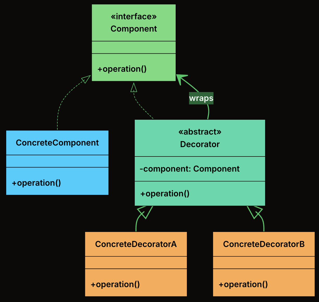
Component: Declares the common interface that both the core object and all decorators implement.
ConcreteComponent: The base object that can be wrapped with decorators. It provides the default behavior.
Decorator: An abstract class that implements the Component interface and holds a reference to another Component. It forwards calls to the wrapped object.
ConcreteDecorator: Extend the base decorator to add new functionality before/after calling the wrapped component’s method.

🛠 Implementation

Define the Component Interface

interface TextView {
    void render();
}

Implement the Concrete Component

class PlainTextView implements TextView {
    private final String text;

    public PlainTextView(String text) {
        this.text = text;
    }

    @Override
    public void render() {
        System.out.print(text);
    }
}

Create the Abstract Decorator

abstract class TextDecorator implements TextView {
    protected final TextView inner;

    public TextDecorator(TextView inner) {
        this.inner = inner;
    }
}

Implement Concrete Decorators

Bold Decorator

class BoldDecorator extends TextDecorator {
    public BoldDecorator(TextView inner) {
        super(inner);
    }

    @Override
    public void render() {
        System.out.print("<b>");
        inner.render();
        System.out.print("</b>");
    }
}

Italic Decorator

class ItalicDecorator extends TextDecorator {
    public ItalicDecorator(TextView inner) {
        super(inner);
    }

    @Override
    public void render() {
        System.out.print("<i>");
        inner.render();
        System.out.print("</i>");
    }
}

Underline Decorator

class UnderlineDecorator extends TextDecorator {
    public UnderlineDecorator(TextView inner) {
        super(inner);
    }

    @Override
    public void render() {
        System.out.print("<u>");
        inner.render();
        System.out.print("</u>");
    }
}

Client Code

public class TextRendererApp {
    public static void main(String[] args) {
        TextView text = new PlainTextView("Hello, World!");

        // Plain text
        System.out.print("Plain:                   ");
        text.render();
        System.out.println();

        // Single decorator: Bold
        System.out.print("Bold:                    ");
        TextView boldText = new BoldDecorator(text);
        boldText.render();
        System.out.println();

        // Two decorators: Italic + Underline
        System.out.print("Italic + Underline:      ");
        TextView italicUnderline = new UnderlineDecorator(new ItalicDecorator(text));
        italicUnderline.render();
        System.out.println();

        // Three decorators: Bold + Italic + Underline
        System.out.print("Bold + Italic + Underline: ");
        TextView allStyles = new UnderlineDecorator(
            new ItalicDecorator(new BoldDecorator(text)));
        allStyles.render();
        System.out.println();
    }
}

Output

Plain:                   Hello, World!
Bold:                    <b>Hello, World!</b>
Italic + Underline:      <u><i>Hello, World!</i></u>
Bold + Italic + Underline: <u><i><b>Hello, World!</b></i></u>

Define the Component Interface

from abc import ABC, abstractmethod

class TextView(ABC):
    @abstractmethod
    def render(self):
        pass

Implement the Concrete Component

class PlainTextView(TextView):
   def __init__(self, text):
       self.text = text

   def render(self):
       print(self.text, end="")

Create the Abstract Decorator

class TextDecorator(TextView):
   def __init__(self, inner):
       self.inner = inner

Implement Concrete Decorators

Bold Decorator

class BoldDecorator(TextDecorator):
   def __init__(self, inner):
       super().__init__(inner)

   def render(self):
       print("<b>", end="")
       self.inner.render()
       print("</b>", end="")

Italic Decorator

class ItalicDecorator(TextDecorator):
   def __init__(self, inner):
       super().__init__(inner)

   def render(self):
       print("<i>", end="")
       self.inner.render()
       print("</i>", end="")

Underline Decorator

class UnderlineDecorator(TextDecorator):
   def __init__(self, inner):
       super().__init__(inner)

   def render(self):
       print("<u>", end="")
       self.inner.render()
       print("</u>", end="")

Client Code

def main():
    text = PlainTextView("Hello, World!")

    # Plain text
    print("Plain:                   ", end="")
    text.render()
    print()

    # Single decorator: Bold
    print("Bold:                    ", end="")
    bold_text = BoldDecorator(text)
    bold_text.render()
    print()

    # Two decorators: Italic + Underline
    print("Italic + Underline:      ", end="")
    italic_underline = UnderlineDecorator(ItalicDecorator(text))
    italic_underline.render()
    print()

    # Three decorators: Bold + Italic + Underline
    print("Bold + Italic + Underline: ", end="")
    all_styles = UnderlineDecorator(ItalicDecorator(BoldDecorator(text)))
    all_styles.render()
    print()


if __name__ == "__main__":
    main()

Output

Plain:                   Hello, World!
Bold:                    <b>Hello, World!</b>
Italic + Underline:      <u><i>Hello, World!</i></u>
Bold + Italic + Underline: <u><i><b>Hello, World!</b></i></u>

Define the Component Interface

class TextView {
public:
   virtual void render() = 0;
   virtual ~TextView() {}
};

Implement the Concrete Component

class PlainTextView : public TextView {
private:
   string text;

public:
   PlainTextView(string text) : text(text) {}

   void render() override {
       cout << text;
   }
};

Create the Abstract Decorator

class TextDecorator : public TextView {
protected:
   TextView* inner;

public:
   TextDecorator(TextView* inner) : inner(inner) {}
};

Implement Concrete Decorators

Bold Decorator

class BoldDecorator : public TextDecorator {
public:
   BoldDecorator(TextView* inner) : TextDecorator(inner) {}

   void render() override {
       cout << "<b>";
       inner->render();
       cout << "</b>";
   }
};

Italic Decorator

class ItalicDecorator : public TextDecorator {
public:
   ItalicDecorator(TextView* inner) : TextDecorator(inner) {}

   void render() override {
       cout << "<i>";
       inner->render();
       cout << "</i>";
   }
};

Underline Decorator

class UnderlineDecorator : public TextDecorator {
public:
   UnderlineDecorator(TextView* inner) : TextDecorator(inner) {}

   void render() override {
       cout << "<u>";
       inner->render();
       cout << "</u>";
   }
};

Client Code

int main() {
    PlainTextView text("Hello, World!");

    // Plain text
    cout << "Plain:                   ";
    text.render();
    cout << endl;

    // Single decorator: Bold
    cout << "Bold:                    ";
    BoldDecorator boldText(&text);
    boldText.render();
    cout << endl;

    // Two decorators: Italic + Underline
    cout << "Italic + Underline:      ";
    ItalicDecorator italic(&text);
    UnderlineDecorator italicUnderline(&italic);
    italicUnderline.render();
    cout << endl;

    // Three decorators: Bold + Italic + Underline
    cout << "Bold + Italic + Underline: ";
    BoldDecorator bold(&text);
    ItalicDecorator italicBold(&bold);
    UnderlineDecorator allStyles(&italicBold);
    allStyles.render();
    cout << endl;

    return 0;
}

Output

Plain:                   Hello, World!
Bold:                    <b>Hello, World!</b>
Italic + Underline:      <u><i>Hello, World!</i></u>
Bold + Italic + Underline: <u><i><b>Hello, World!</b></i></u>

Define the Component Interface

interface ITextView
{
   void Render();
}

Implement the Concrete Component

class PlainTextView : ITextView
{
   private readonly string text;

   public PlainTextView(string text)
   {
       this.text = text;
   }

   public void Render()
   {
       Console.Write(text);
   }
}

Create the Abstract Decorator

abstract class TextDecorator : ITextView
{
   protected readonly ITextView inner;

   public TextDecorator(ITextView inner)
   {
       this.inner = inner;
   }

   public abstract void Render();
}

Implement Concrete Decorators

Bold Decorator

class BoldDecorator : TextDecorator
{
   public BoldDecorator(ITextView inner) : base(inner)
   {
   }

   public override void Render()
   {
       Console.Write("<b>");
       inner.Render();
       Console.Write("</b>");
   }
}

Italic Decorator

class ItalicDecorator : TextDecorator
{
   public ItalicDecorator(ITextView inner) : base(inner)
   {
   }

   public override void Render()
   {
       Console.Write("<i>");
       inner.Render();
       Console.Write("</i>");
   }
}

Underline Decorator

class UnderlineDecorator : TextDecorator
{
   public UnderlineDecorator(ITextView inner) : base(inner)
   {
   }

   public override void Render()
   {
       Console.Write("<u>");
       inner.Render();
       Console.Write("</u>");
   }
}

Client Code

public class TextRendererApp
{
    public static void Main()
    {
        ITextView text = new PlainTextView("Hello, World!");

        // Plain text
        Console.Write("Plain:                   ");
        text.Render();
        Console.WriteLine();

        // Single decorator: Bold
        Console.Write("Bold:                    ");
        ITextView boldText = new BoldDecorator(text);
        boldText.Render();
        Console.WriteLine();

        // Two decorators: Italic + Underline
        Console.Write("Italic + Underline:      ");
        ITextView italicUnderline = new UnderlineDecorator(new ItalicDecorator(text));
        italicUnderline.Render();
        Console.WriteLine();

        // Three decorators: Bold + Italic + Underline
        Console.Write("Bold + Italic + Underline: ");
        ITextView allStyles = new UnderlineDecorator(
            new ItalicDecorator(new BoldDecorator(text)));
        allStyles.Render();
        Console.WriteLine();
    }
}

Output

Plain:                   Hello, World!
Bold:                    <b>Hello, World!</b>
Italic + Underline:      <u><i>Hello, World!</i></u>
Bold + Italic + Underline: <u><i><b>Hello, World!</b></i></u>

Define the Component Interface

interface TextView {
  render(): void;
}

Implement the Concrete Component

class PlainTextView implements TextView {
  private readonly text: string;

  constructor(text: string) {
    this.text = text;
  }

  render(): void {
    process.stdout.write(this.text);
  }
}

Create the Abstract Decorator

abstract class TextDecorator implements TextView {
  protected readonly inner: TextView;

  constructor(inner: TextView) {
    this.inner = inner;
  }

  abstract render(): void;
}

Implement Concrete Decorators

Bold Decorator

class BoldDecorator extends TextDecorator {
  constructor(inner: TextView) {
    super(inner);
  }

  render(): void {
    process.stdout.write("<b>");
    this.inner.render();
    process.stdout.write("</b>");
  }
}

Italic Decorator

class ItalicDecorator extends TextDecorator {
  constructor(inner: TextView) {
    super(inner);
  }

  render(): void {
    process.stdout.write("<i>");
    this.inner.render();
    process.stdout.write("</i>");
  }
}

Underline Decorator

class UnderlineDecorator extends TextDecorator {
  constructor(inner: TextView) {
    super(inner);
  }

  render(): void {
    process.stdout.write("<u>");
    this.inner.render();
    process.stdout.write("</u>");
  }
}

Client Code

const text: TextView = new PlainTextView("Hello, World!");

// Plain text
process.stdout.write("Plain:                   ");
text.render();
console.log();

// Single decorator: Bold
process.stdout.write("Bold:                    ");
const boldText: TextView = new BoldDecorator(text);
boldText.render();
console.log();

// Two decorators: Italic + Underline
process.stdout.write("Italic + Underline:      ");
const italicUnderline: TextView = new UnderlineDecorator(
  new ItalicDecorator(text),
);
italicUnderline.render();
console.log();

// Three decorators: Bold + Italic + Underline
process.stdout.write("Bold + Italic + Underline: ");
const allStyles: TextView = new UnderlineDecorator(
  new ItalicDecorator(new BoldDecorator(text)),
);
allStyles.render();
console.log();

Output

Plain:                   Hello, World!
Bold:                    <b>Hello, World!</b>
Italic + Underline:      <u><i>Hello, World!</i></u>
Bold + Italic + Underline: <u><i><b>Hello, World!</b></i></u>

Composite

📖 Definition

The Composite Design Pattern is a structural pattern that lets you treat individual objects and compositions of objects uniformly.

It allows you to build tree-like structures (e.g., file systems, UI hierarchies, organizational charts) where clients can work with both single elements and groups of elements using the same interface.

It’s particularly useful in situations where:

You need to represent part-whole hierarchies.
You want to perform operations on both leaf nodes and composite nodes in a consistent way.
You want to avoid writing special-case logic to distinguish between “single” and “grouped” objects.

🧩 Class Diagram

Composite Pattern Class Diagram

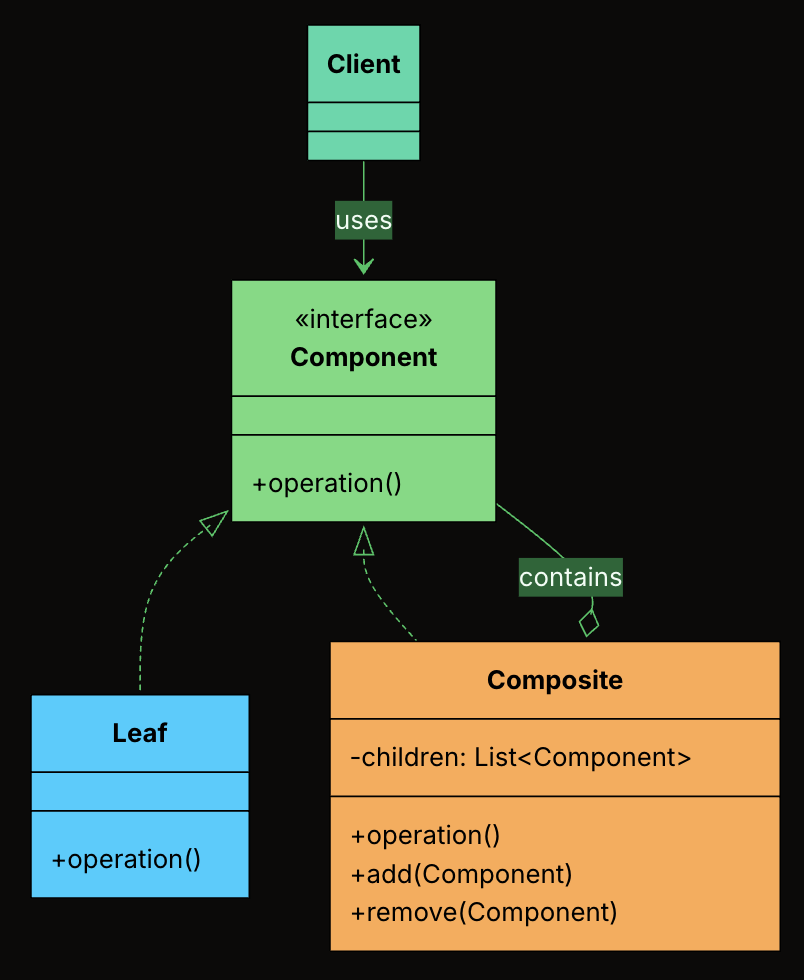
Component Interface: The shared interface that declares operations common to both leaves and composites.
Leaf: An end object in the tree that has no children. It implements the Component interface directly.
Composite: A container that holds child Components and implements the Component interface by delegating to its children.
Client: Works with the tree through the Component interface, without knowing whether it holds a leaf or a composite.

🛠 Implementation

Define the Component Interface

interface FileSystemItem {
    int getSize();
    void printStructure(String indent);
    void delete();
}

Create the Leaf Class

class File implements FileSystemItem {
    private final String name;
    private final int size;

    public File(String name, int size) {
        this.name = name;
        this.size = size;
    }

    @Override
    public int getSize() {
        return size;
    }

    @Override
    public void printStructure(String indent) {
        System.out.println(indent + "- " + name + " (" + size + " KB)");
    }

    @Override
    public void delete() {
        System.out.println("Deleting file: " + name);
    }
}

Create the Composite Class

class Folder implements FileSystemItem {
    private final String name;
    private final List<FileSystemItem> children = new ArrayList<>();

    public Folder(String name) {
        this.name = name;
    }

    public void addItem(FileSystemItem item) {
        children.add(item);
    }

    public void removeItem(FileSystemItem item) {
        children.remove(item);
    }

    @Override
    public int getSize() {
        int total = 0;
        for (FileSystemItem item : children) {
            total += item.getSize();
        }
        return total;
    }

    @Override
    public void printStructure(String indent) {
        System.out.println(indent + "+ " + name + "/");
        for (FileSystemItem item : children) {
            item.printStructure(indent + "  ");
        }
    }

    @Override
    public void delete() {
        for (FileSystemItem item : children) {
            item.delete();
        }
        System.out.println("Deleting folder: " + name);
    }
}

Client Code

public class FileExplorerApp {
    public static void main(String[] args) {
        FileSystemItem file1 = new File("readme.txt", 5);
        FileSystemItem file2 = new File("photo.jpg", 1500);
        FileSystemItem file3 = new File("data.csv", 300);

        Folder documents = new Folder("Documents");
        documents.addItem(file1);
        documents.addItem(file3);

        Folder pictures = new Folder("Pictures");
        pictures.addItem(file2);

        Folder home = new Folder("Home");
        home.addItem(documents);
        home.addItem(pictures);

        System.out.println("---- File Structure ----");
        home.printStructure("");

        System.out.println("\nTotal Size: " + home.getSize() + " KB");

        System.out.println("\n---- Deleting All ----");
        home.delete();
    }
}

Output

---- File Structure ----
+ Home/
  + Documents/
    - readme.txt (5 KB)
    - data.csv (300 KB)
  + Pictures/
    - photo.jpg (1500 KB)

Total Size: 1805 KB

---- Deleting All ----
Deleting file: readme.txt
Deleting file: data.csv
Deleting folder: Documents
Deleting file: photo.jpg
Deleting folder: Pictures
Deleting folder: Home

Define the Component Interface

from abc import ABC, abstractmethod

class FileSystemItem(ABC):
    @abstractmethod
    def get_size(self) -> int:
        pass

    @abstractmethod
    def print_structure(self, indent: str):
        pass

    @abstractmethod
    def delete(self):
        pass

Create the Leaf Class

class File(FileSystemItem):
    def __init__(self, name: str, size: int):
        self.name = name
        self.size = size

    def get_size(self) -> int:
        return self.size

    def print_structure(self, indent: str):
        print(f"{indent}- {self.name} ({self.size} KB)")

    def delete(self):
        print(f"Deleting file: {self.name}")

Create the Composite Class

class Folder(FileSystemItem):
    def __init__(self, name: str):
        self.name = name
        self.children: list[FileSystemItem] = []

    def add_item(self, item: FileSystemItem):
        self.children.append(item)

    def remove_item(self, item: FileSystemItem):
        self.children.remove(item)

    def get_size(self) -> int:
        total = 0
        for item in self.children:
            total += item.get_size()
        return total

    def print_structure(self, indent: str):
        print(f"{indent}+ {self.name}/")
        for item in self.children:
            item.print_structure(indent + "  ")

    def delete(self):
        for item in self.children:
            item.delete()
        print(f"Deleting folder: {self.name}")

Client Code

if __name__ == "__main__":
    file1 = File("readme.txt", 5)
    file2 = File("photo.jpg", 1500)
    file3 = File("data.csv", 300)

    documents = Folder("Documents")
    documents.add_item(file1)
    documents.add_item(file3)

    pictures = Folder("Pictures")
    pictures.add_item(file2)

    home = Folder("Home")
    home.add_item(documents)
    home.add_item(pictures)

    print("---- File Structure ----")
    home.print_structure("")

    print(f"\nTotal Size: {home.get_size()} KB")

    print("\n---- Deleting All ----")
    home.delete()

Output

---- File Structure ----
+ Home/
  + Documents/
    - readme.txt (5 KB)
    - data.csv (300 KB)
  + Pictures/
    - photo.jpg (1500 KB)

Total Size: 1805 KB

---- Deleting All ----
Deleting file: readme.txt
Deleting file: data.csv
Deleting folder: Documents
Deleting file: photo.jpg
Deleting folder: Pictures
Deleting folder: Home

Define the Component Interface

class FileSystemItem {
public:
    virtual int getSize() = 0;
    virtual void printStructure(string indent) = 0;
    virtual void deleteItem() = 0;
    virtual ~FileSystemItem() {}
};

Create the Leaf Class

class File : public FileSystemItem {
private:
    string name;
    int size;

public:
    File(string name, int size) : name(name), size(size) {}

    int getSize() override {
        return size;
    }

    void printStructure(string indent) override {
        cout << indent << "- " << name << " (" << size << " KB)" << endl;
    }

    void deleteItem() override {
        cout << "Deleting file: " << name << endl;
    }
};

Create the Composite Class

class Folder : public FileSystemItem {
private:
    string name;
    vector<FileSystemItem*> children;

public:
    Folder(string name) : name(name) {}

    void addItem(FileSystemItem* item) {
        children.push_back(item);
    }

    void removeItem(FileSystemItem* item) {
        children.erase(
            remove(children.begin(), children.end(), item),
            children.end()
        );
    }

    int getSize() override {
        int total = 0;
        for (FileSystemItem* item : children) {
            total += item->getSize();
        }
        return total;
    }

    void printStructure(string indent) override {
        cout << indent << "+ " << name << "/" << endl;
        for (FileSystemItem* item : children) {
            item->printStructure(indent + "  ");
        }
    }

    void deleteItem() override {
        for (FileSystemItem* item : children) {
            item->deleteItem();
        }
        cout << "Deleting folder: " << name << endl;
    }
};

Client Code

int main() {
    FileSystemItem* file1 = new File("readme.txt", 5);
    FileSystemItem* file2 = new File("photo.jpg", 1500);
    FileSystemItem* file3 = new File("data.csv", 300);

    Folder* documents = new Folder("Documents");
    documents->addItem(file1);
    documents->addItem(file3);

    Folder* pictures = new Folder("Pictures");
    pictures->addItem(file2);

    Folder* home = new Folder("Home");
    home->addItem(documents);
    home->addItem(pictures);

    cout << "---- File Structure ----" << endl;
    home->printStructure("");

    cout << "\nTotal Size: " << home->getSize() << " KB" << endl;

    cout << "\n---- Deleting All ----" << endl;
    home->deleteItem();

    delete file1;
    delete file2;
    delete file3;
    delete documents;
    delete pictures;
    delete home;

    return 0;
}

Output

---- File Structure ----
+ Home/
  + Documents/
    - readme.txt (5 KB)
    - data.csv (300 KB)
  + Pictures/
    - photo.jpg (1500 KB)

Total Size: 1805 KB

---- Deleting All ----
Deleting file: readme.txt
Deleting file: data.csv
Deleting folder: Documents
Deleting file: photo.jpg
Deleting folder: Pictures
Deleting folder: Home

Define the Component Interface

interface IFileSystemItem
{
    int GetSize();
    void PrintStructure(string indent);
    void Delete();
}

Create the Leaf Class

class File : IFileSystemItem
{
    private readonly string name;
    private readonly int size;

    public File(string name, int size)
    {
        this.name = name;
        this.size = size;
    }

    public int GetSize() {
        return size;
    }

    public void PrintStructure(string indent)
    {
        Console.WriteLine(indent + "- " + name + " (" + size + " KB)");
    }

    public void Delete()
    {
        Console.WriteLine("Deleting file: " + name);
    }
}

Create the Composite Class

class Folder : IFileSystemItem
{
    private readonly string name;
    private readonly List<IFileSystemItem> children = new List<IFileSystemItem>();

    public Folder(string name) {
        this.name = name;
    }

    public void AddItem(IFileSystemItem item) {
        children.Add(item);
    }

    public void RemoveItem(IFileSystemItem item) {
        children.Remove(item);
    }

    public int GetSize()
    {
        int total = 0;
        foreach (IFileSystemItem item in children)
        {
            total += item.GetSize();
        }
        return total;
    }

    public void PrintStructure(string indent)
    {
        Console.WriteLine(indent + "+ " + name + "/");
        foreach (IFileSystemItem item in children)
        {
            item.PrintStructure(indent + "  ");
        }
    }

    public void Delete()
    {
        foreach (IFileSystemItem item in children)
        {
            item.Delete();
        }
        Console.WriteLine("Deleting folder: " + name);
    }
}

Client Code

public class Program
{
    public static void Main()
    {
        IFileSystemItem file1 = new File("readme.txt", 5);
        IFileSystemItem file2 = new File("photo.jpg", 1500);
        IFileSystemItem file3 = new File("data.csv", 300);

        Folder documents = new Folder("Documents");
        documents.AddItem(file1);
        documents.AddItem(file3);

        Folder pictures = new Folder("Pictures");
        pictures.AddItem(file2);

        Folder home = new Folder("Home");
        home.AddItem(documents);
        home.AddItem(pictures);

        Console.WriteLine("---- File Structure ----");
        home.PrintStructure("");

        Console.WriteLine("\nTotal Size: " + home.GetSize() + " KB");

        Console.WriteLine("\n---- Deleting All ----");
        home.Delete();
    }
}

Output

---- File Structure ----
+ Home/
  + Documents/
    - readme.txt (5 KB)
    - data.csv (300 KB)
  + Pictures/
    - photo.jpg (1500 KB)

Total Size: 1805 KB

---- Deleting All ----
Deleting file: readme.txt
Deleting file: data.csv
Deleting folder: Documents
Deleting file: photo.jpg
Deleting folder: Pictures
Deleting folder: Home

Define the Component Interface

interface FileSystemItem {
  getSize(): number;
  printStructure(indent: string): void;
  delete(): void;
}

Create the Leaf Class

class FileNode implements FileSystemItem {
  private readonly name: string;
  private readonly size: number;

  constructor(name: string, size: number) {
    this.name = name;
    this.size = size;
  }

  getSize(): number {
    return this.size;
  }

  printStructure(indent: string): void {
    console.log(indent + "- " + this.name + " (" + this.size + " KB)");
  }

  delete(): void {
    console.log("Deleting file: " + this.name);
  }
}

Create the Composite Class

class FolderNode implements FileSystemItem {
  private readonly name: string;
  private readonly children: FileSystemItem[] = [];

  constructor(name: string) {
    this.name = name;
  }

  addItem(item: FileSystemItem): void {
    this.children.push(item);
  }

  removeItem(item: FileSystemItem): void {
    const index = this.children.indexOf(item);
    if (index !== -1) {
      this.children.splice(index, 1);
    }
  }

  getSize(): number {
    let total = 0;
    for (const item of this.children) {
      total += item.getSize();
    }
    return total;
  }

  printStructure(indent: string): void {
    console.log(indent + "+ " + this.name + "/");
    for (const item of this.children) {
      item.printStructure(indent + "  ");
    }
  }

  delete(): void {
    for (const item of this.children) {
      item.delete();
    }
    console.log("Deleting folder: " + this.name);
  }
}

Client Code

const file1: FileSystemItem = new FileNode("readme.txt", 5);
const file2: FileSystemItem = new FileNode("photo.jpg", 1500);
const file3: FileSystemItem = new FileNode("data.csv", 300);

const documents = new FolderNode("Documents");
documents.addItem(file1);
documents.addItem(file3);

const pictures = new FolderNode("Pictures");
pictures.addItem(file2);

const home = new FolderNode("Home");
home.addItem(documents);
home.addItem(pictures);

console.log("---- File Structure ----");
home.printStructure("");

console.log("\nTotal Size: " + home.getSize() + " KB");

console.log("\n---- Deleting All ----");
home.delete();

Output

---- File Structure ----
+ Home/
  + Documents/
    - readme.txt (5 KB)
    - data.csv (300 KB)
  + Pictures/
    - photo.jpg (1500 KB)

Total Size: 1805 KB

---- Deleting All ----
Deleting file: readme.txt
Deleting file: data.csv
Deleting folder: Documents
Deleting file: photo.jpg
Deleting folder: Pictures
Deleting folder: Home

Facade

📖 Definition

The Facade Design Pattern is a structural design pattern that provides a single, simplified interface to a complex subsystem. Instead of forcing clients to coordinate many moving parts, a facade hides the internal complexity and exposes a clean, easy-to-use entry point.

It’s particularly useful in situations where:

Your system contains many interdependent classes or low-level APIs.
The client doesn’t need to know how those parts work internally.
You want to reduce coupling and make the system easier to learn and use.

🧩 Class Diagram

Facade Pattern Class Diagram

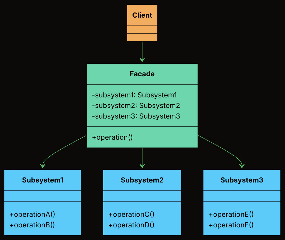
Facade: Knows which subsystem classes to use and in what order. Delegates requests to appropriate subsystem methods without exposing internal details to the client.
Subsystem Classes: Provides the actual business logic to handle a specific task. Do not know about the facade. Can still be used independently if needed.
Client: Uses the Facade to initiate a deployment, instead of interacting with the subsystem classes directly.

🛠 Implementation

Define Facade Class

class DeploymentFacade {
    private VersionControlSystem vcs = new VersionControlSystem();
    private BuildSystem buildSystem = new BuildSystem();
    private TestingFramework testingFramework = new TestingFramework();
    private DeploymentTarget deploymentTarget = new DeploymentTarget();

    public boolean deployApplication(String branch, String serverAddress) {
        System.out.println("\nFACADE: --- Initiating FULL DEPLOYMENT for branch: " + branch + " to " + serverAddress + " ---");
        boolean success = true;

        try {
            vcs.pullLatestChanges(branch);

            if (!buildSystem.compileProject()) {
                System.err.println("FACADE: DEPLOYMENT FAILED - Build compilation failed.");
                return false;
            }

            String artifactPath = buildSystem.getArtifactPath();

            if (!testingFramework.runUnitTests()) {
                System.err.println("FACADE: DEPLOYMENT FAILED - Unit tests failed.");
                return false;
            }

            if (!testingFramework.runIntegrationTests()) {
                System.err.println("FACADE: DEPLOYMENT FAILED - Integration tests failed.");
                return false;
            }

            deploymentTarget.transferArtifact(artifactPath, serverAddress);
            deploymentTarget.activateNewVersion(serverAddress);

            System.out.println("FACADE: APPLICATION DEPLOYED SUCCESSFULLY to " + serverAddress + "!");
        } catch (Exception e) {
            System.err.println("FACADE: DEPLOYMENT FAILED - An unexpected error occurred: " + e.getMessage());
            e.printStackTrace();
            success = false;
        }

        return success;
    }
}

Client Code

public class DeploymentAppFacade {
    public static void main(String[] args) {
        DeploymentFacade deploymentFacade = new DeploymentFacade();

        // Deploy to production
        deploymentFacade.deployApplication("main", "prod.server.example.com");

        // Deploy a feature branch to staging
        System.out.println("\n--- Deploying feature branch to staging ---");
        deploymentFacade.deployApplication("feature/new-ui", "staging.server.example.com");
    }
}

Define Facade Class

class DeploymentFacade:
   def __init__(self):
       self.vcs = VersionControlSystem()
       self.build_system = BuildSystem()
       self.testing_framework = TestingFramework()
       self.deployment_target = DeploymentTarget()

   def deploy_application(self, branch, server_address):
       print(f"\nFACADE: --- Initiating FULL DEPLOYMENT for branch: {branch} to {server_address} ---")
       success = True

       try:
           self.vcs.pull_latest_changes(branch)

           if not self.build_system.compile_project():
               print("FACADE: DEPLOYMENT FAILED - Build compilation failed.", file=sys.stderr)
               return False

           artifact_path = self.build_system.get_artifact_path()

           if not self.testing_framework.run_unit_tests():
               print("FACADE: DEPLOYMENT FAILED - Unit tests failed.", file=sys.stderr)
               return False

           if not self.testing_framework.run_integration_tests():
               print("FACADE: DEPLOYMENT FAILED - Integration tests failed.", file=sys.stderr)
               return False

           self.deployment_target.transfer_artifact(artifact_path, server_address)
           self.deployment_target.activate_new_version(server_address)

           print(f"FACADE: APPLICATION DEPLOYED SUCCESSFULLY to {server_address}!")
       except Exception as e:
           print(f"FACADE: DEPLOYMENT FAILED - An unexpected error occurred: {str(e)}", file=sys.stderr)
           import traceback
           traceback.print_exc()
           success = False

       return success

Client Code

class DeploymentAppFacade:
   @staticmethod
   def main():
       deployment_facade = DeploymentFacade()

       # Deploy to production
       deployment_facade.deploy_application("main", "prod.server.example.com")

       # Deploy a feature branch to staging
       print("\n--- Deploying feature branch to staging ---")
       deployment_facade.deploy_application("feature/new-ui", "staging.server.example.com")

if __name__ == "__main__":
   DeploymentAppFacade.main()

Define Facade Class

class DeploymentFacade {
private:
   VersionControlSystem vcs;
   BuildSystem buildSystem;
   TestingFramework testingFramework;
   DeploymentTarget deploymentTarget;

public:
   bool deployApplication(string branch, string serverAddress) {
       cout << "\nFACADE: --- Initiating FULL DEPLOYMENT for branch: " << branch << " to " << serverAddress << " ---" << endl;
       bool success = true;

       try {
           vcs.pullLatestChanges(branch);

           if (!buildSystem.compileProject()) {
               cerr << "FACADE: DEPLOYMENT FAILED - Build compilation failed." << endl;
               return false;
           }

           string artifactPath = buildSystem.getArtifactPath();

           if (!testingFramework.runUnitTests()) {
               cerr << "FACADE: DEPLOYMENT FAILED - Unit tests failed." << endl;
               return false;
           }

           if (!testingFramework.runIntegrationTests()) {
               cerr << "FACADE: DEPLOYMENT FAILED - Integration tests failed." << endl;
               return false;
           }

           deploymentTarget.transferArtifact(artifactPath, serverAddress);
           deploymentTarget.activateNewVersion(serverAddress);

           cout << "FACADE: APPLICATION DEPLOYED SUCCESSFULLY to " << serverAddress << "!" << endl;
       } catch (exception& e) {
           cerr << "FACADE: DEPLOYMENT FAILED - An unexpected error occurred: " << e.what() << endl;
           success = false;
       }

       return success;
   }
};

Client Code

class DeploymentAppFacade {
public:
   static void main() {
       DeploymentFacade deploymentFacade;

       // Deploy to production
       deploymentFacade.deployApplication("main", "prod.server.example.com");

       // Deploy a feature branch to staging
       cout << "\n--- Deploying feature branch to staging ---" << endl;
       deploymentFacade.deployApplication("feature/new-ui", "staging.server.example.com");
   }
};

int main() {
   DeploymentAppFacade::main();
   return 0;
}

Define Facade Class

class DeploymentFacade
{
   private VersionControlSystem vcs = new VersionControlSystem();
   private BuildSystem buildSystem = new BuildSystem();
   private TestingFramework testingFramework = new TestingFramework();
   private DeploymentTarget deploymentTarget = new DeploymentTarget();

   public bool DeployApplication(string branch, string serverAddress)
   {
       Console.WriteLine($"\nFACADE: --- Initiating FULL DEPLOYMENT for branch: {branch} to {serverAddress} ---");
       bool success = true;

       try
       {
           vcs.PullLatestChanges(branch);

           if (!buildSystem.CompileProject())
           {
               Console.Error.WriteLine("FACADE: DEPLOYMENT FAILED - Build compilation failed.");
               return false;
           }

           string artifactPath = buildSystem.GetArtifactPath();

           if (!testingFramework.RunUnitTests())
           {
               Console.Error.WriteLine("FACADE: DEPLOYMENT FAILED - Unit tests failed.");
               return false;
           }

           if (!testingFramework.RunIntegrationTests())
           {
               Console.Error.WriteLine("FACADE: DEPLOYMENT FAILED - Integration tests failed.");
               return false;
           }

           deploymentTarget.TransferArtifact(artifactPath, serverAddress);
           deploymentTarget.ActivateNewVersion(serverAddress);

           Console.WriteLine($"FACADE: APPLICATION DEPLOYED SUCCESSFULLY to {serverAddress}!");
       }
       catch (Exception e)
       {
           Console.Error.WriteLine($"FACADE: DEPLOYMENT FAILED - An unexpected error occurred: {e.Message}");
           Console.Error.WriteLine(e.StackTrace);
           success = false;
       }

       return success;
   }
}

Client Code

public class DeploymentAppFacade
{
   public static void Main(string[] args)
   {
       DeploymentFacade deploymentFacade = new DeploymentFacade();

       // Deploy to production
       deploymentFacade.DeployApplication("main", "prod.server.example.com");

       // Deploy a feature branch to staging
       Console.WriteLine("\n--- Deploying feature branch to staging ---");
       deploymentFacade.DeployApplication("feature/new-ui", "staging.server.example.com");
   }
}

Define Facade Class

class DeploymentFacade {
  private vcs = new VersionControlSystem();
  private buildSystem = new BuildSystem();
  private testingFramework = new TestingFramework();
  private deploymentTarget = new DeploymentTarget();

  deployApplication(branch: string, serverAddress: string): boolean {
    console.log(
      "\nFACADE: --- Initiating FULL DEPLOYMENT for branch: " +
        branch +
        " to " +
        serverAddress +
        " ---",
    );
    let success = true;

    try {
      this.vcs.pullLatestChanges(branch);

      if (!this.buildSystem.compileProject()) {
        console.error("FACADE: DEPLOYMENT FAILED - Build compilation failed.");
        return false;
      }

      const artifactPath = this.buildSystem.getArtifactPath();

      if (!this.testingFramework.runUnitTests()) {
        console.error("FACADE: DEPLOYMENT FAILED - Unit tests failed.");
        return false;
      }

      if (!this.testingFramework.runIntegrationTests()) {
        console.error("FACADE: DEPLOYMENT FAILED - Integration tests failed.");
        return false;
      }

      this.deploymentTarget.transferArtifact(artifactPath, serverAddress);
      this.deploymentTarget.activateNewVersion(serverAddress);

      console.log(
        "FACADE: APPLICATION DEPLOYED SUCCESSFULLY to " + serverAddress + "!",
      );
    } catch (e) {
      console.error(
        "FACADE: DEPLOYMENT FAILED - An unexpected error occurred: " +
          (e as Error).message,
      );
      console.error(e);
      success = false;
    }

    return success;
  }
}

Client Code

class DeploymentAppFacade {
  static main(): void {
    const deploymentFacade = new DeploymentFacade();

    // Deploy to production
    deploymentFacade.deployApplication("main", "prod.server.example.com");

    // Deploy a feature branch to staging
    console.log("\n--- Deploying feature branch to staging ---");
    deploymentFacade.deployApplication(
      "feature/new-ui",
      "staging.server.example.com",
    );
  }
}

Behavioral Patterns

Iterator
Strategy
Observer

Iterator

📖 Definition

The Iterator Design Pattern is a behavioral pattern that provides a standard way to access elements of a collection sequentially without exposing its internal structure.

At its core, the Iterator pattern is about separating the logic of how you move through a collection from the collection itself. Instead of letting clients directly access internal arrays, lists, or other data structures, the collection provides an iterator object that handles traversal.

It’s particularly useful in situations where:

You need to traverse a collection (like a list, tree, or graph) in a consistent and flexible way.
You want to support multiple ways to iterate (e.g., forward, backward, filtering, or skipping elements).
You want to decouple traversal logic from collection structure, so the client doesn’t depend on the internal representation.

🧩 Class Diagram

Iterator Pattern Class Diagram

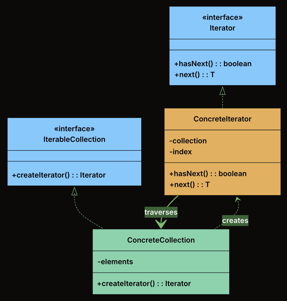
Iterator (interface): Declares the operations required to traverse a collection. At minimum, this includes hasNext() to check if more elements exist, and next() to retrieve the next element.
ConcreteIterator: Implements the Iterator interface for a specific collection. It maintains the current position within the collection and knows how to move to the next element.
IterableCollection (interface): Declares a method for creating an iterator. Any class implementing this interface promises it can be iterated.
ConcreteCollection: Implements the IterableCollection interface. It stores elements and returns an appropriate iterator when asked.

🛠 Implementation

Define the Iterator Interface

interface Iterator<T> {
    boolean hasNext();
    T next();
}

Define the IterableCollection Interface

interface IterableCollection<T> {
    Iterator<T> createIterator();
}

Implement the Concrete Collection

class Playlist implements IterableCollection<String> {
    private final List<String> songs = new ArrayList<>();

    public void addSong(String song) {
        songs.add(song);
    }

    public String getSongAt(int index) {
        return songs.get(index);
    }

    public int getSize() {
        return songs.size();
    }

    @Override
    public Iterator<String> createIterator() {
        return new PlaylistIterator(this);
    }
}

Implement the Concrete Iterator

class PlaylistIterator implements Iterator<String> {
    private final Playlist playlist;
    private int index = 0;

    public PlaylistIterator(Playlist playlist) {
        this.playlist = playlist;
    }

    @Override
    public boolean hasNext() {
        return index < playlist.getSize();
    }

    @Override
    public String next() {
        return playlist.getSongAt(index++);
    }
}

Client Code

public class MusicPlayer {
    public static void main(String[] args) {
        Playlist playlist = new Playlist();
        playlist.addSong("Shape of You");
        playlist.addSong("Bohemian Rhapsody");
        playlist.addSong("Blinding Lights");

        Iterator<String> iterator = playlist.createIterator();

        System.out.println("Now Playing:");
        while (iterator.hasNext()) {
            System.out.println(" 🎵 " + iterator.next());
        }
    }
}

Output

Now Playing:
🎵 Shape of You
🎵 Bohemian Rhapsody
🎵 Blinding Lights

Define the Iterator Interface

from abc import ABC, abstractmethod

class Iterator(ABC):
    @abstractmethod
    def has_next(self) -> bool:
        pass

    @abstractmethod
    def next(self):
        pass

Define the IterableCollection Interface

class IterableCollection(ABC):
    @abstractmethod
    def create_iterator(self):
        pass

Implement the Concrete Collection

class Playlist(IterableCollection):
    def __init__(self):
        self.songs = []

    def add_song(self, song):
        self.songs.append(song)

    def get_song_at(self, index):
        return self.songs[index]

    def get_size(self):
        return len(self.songs)

    def create_iterator(self):
        return PlaylistIterator(self)

Implement the Concrete Iterator

class PlaylistIterator(Iterator):
    def __init__(self, playlist):
        self.playlist = playlist
        self.index = 0

    def has_next(self):
        return self.index < self.playlist.get_size()

    def next(self):
        song = self.playlist.get_song_at(self.index)
        self.index += 1
        return song

Client Code

def music_player_demo():
    playlist = PlaylistIteratorPattern()
    playlist.add_song("Shape of You")
    playlist.add_song("Bohemian Rhapsody")
    playlist.add_song("Blinding Lights")

    iterator = playlist.create_iterator()

    print("Now Playing:")
    while iterator.has_next():
        print(f" 🎵 {iterator.next()}")

if __name__ == "__main__":

    music_player_demo()

Output

Now Playing:
🎵 Shape of You
🎵 Bohemian Rhapsody
🎵 Blinding Lights

Define the Iterator Interface

template<typename T>
class Iterator {
public:
    virtual ~Iterator() {}
    virtual bool hasNext() = 0;
    virtual T next() = 0;
};

Define the IterableCollection Interface

template<typename T>
class IterableCollection {
public:
    virtual ~IterableCollection() {}
    virtual Iterator<T>* createIterator() = 0;
};

Implement the Concrete Collection

class Playlist : public IterableCollection<string> {
private:
    vector<string> songs;

public:
    void addSong(const string& song) {
        songs.push_back(song);
    }

    string getSongAt(int index) const {
        return songs[index];
    }

    int getSize() const {
        return songs.size();
    }

    Iterator<string>* createIterator() override {
        return new PlaylistIterator(this);
    }
};

Implement the Concrete Iterator

class PlaylistIterator : public Iterator<string> {
private:
    PlaylistIteratorPattern* playlist;
    int index;

public:
    PlaylistIterator(PlaylistIteratorPattern* pl);

    bool hasNext() override {
      return index < playlist->getSize();
    }

    string next() override {
      string song = playlist->getSongAt(index);
      index++;
      return song;
    }
};

Client Code

void musicPlayerDemo() {
    PlaylistIteratorPattern playlist;
    playlist.addSong("Shape of You");
    playlist.addSong("Bohemian Rhapsody");
    playlist.addSong("Blinding Lights");

    Iterator<string>* iterator = playlist.createIterator();

    cout << "Now Playing:" << endl;
    while (iterator->hasNext()) {
        cout << " 🎵 " << iterator->next() << endl;
    }

    delete iterator;
}

int main() {
    musicPlayerDemo();
    return 0;
}

Output

Now Playing:
🎵 Shape of You
🎵 Bohemian Rhapsody
🎵 Blinding Lights

Define the Iterator Interface

interface IIterator<T>
{
    bool HasNext();
    T Next();
}

Define the IterableCollection Interface

interface IIterableCollection<T>
{
    IIterator<T> CreateIterator();
}

Implement the Concrete Collection

class Playlist : IIterableCollection<string>
{
    private List<string> songs = new List<string>();

    public void AddSong(string song)
    {
        songs.Add(song);
    }

    public string GetSongAt(int index)
    {
        return songs[index];
    }

    public int GetSize()
    {
        return songs.Count;
    }

    public IIterator<string> CreateIterator()
    {
        return new PlaylistIterator(this);
    }
}

Implement the Concrete Iterator

class PlaylistIterator : IIterator<string>
{
    private PlaylistIteratorPattern playlist;
    private int index = 0;

    public PlaylistIterator(PlaylistIteratorPattern playlist)
    {
        this.playlist = playlist;
    }

    public bool HasNext()
    {
        return index < playlist.GetSize();
    }

    public string Next()
    {
        string song = playlist.GetSongAt(index);
        index++;
        return song;
    }
}

Client Code

public class Program
{
    public static void Main(string[] args)
    {
        PlaylistIteratorPattern playlist = new PlaylistIteratorPattern();
        playlist.AddSong("Shape of You");
        playlist.AddSong("Bohemian Rhapsody");
        playlist.AddSong("Blinding Lights");

        IIterator<string> iterator = playlist.CreateIterator();

        Console.WriteLine("Now Playing:");
        while (iterator.HasNext())
        {
            Console.WriteLine($" 🎵 {iterator.Next()}");
        }
    }
}

Output

Now Playing:
🎵 Shape of You
🎵 Bohemian Rhapsody
🎵 Blinding Lights

Define the Iterator Interface

interface Iterator<T> {
  hasNext(): boolean;
  next(): T;
}

Define the IterableCollection Interface

interface IterableCollection<T> {
  createIterator(): Iterator<T>;
}

Implement the Concrete Collection

class Playlist implements IterableCollection<string> {
  private readonly songs: string[] = [];

  addSong(song: string): void {
    this.songs.push(song);
  }

  getSongAt(index: number): string {
    return this.songs[index];
  }

  getSize(): number {
    return this.songs.length;
  }

  createIterator(): Iterator<string> {
    return new PlaylistIterator(this);
  }
}

Implement the Concrete Iterator

class PlaylistIterator implements Iterator<string> {
  private readonly playlist: Playlist;
  private index: number = 0;

  constructor(playlist: Playlist) {
    this.playlist = playlist;
  }

  hasNext(): boolean {
    return this.index < this.playlist.getSize();
  }

  next(): string {
    return this.playlist.getSongAt(this.index++);
  }
}

Client Code

class MusicPlayer {
  static main(): void {
    const playlist = new Playlist();
    playlist.addSong("Shape of You");
    playlist.addSong("Bohemian Rhapsody");
    playlist.addSong("Blinding Lights");

    const iterator: Iterator<string> = playlist.createIterator();

    console.log("Now Playing:");
    while (iterator.hasNext()) {
      console.log(" 🎵 " + iterator.next());
    }
  }
}

Output

Now Playing:
🎵 Shape of You
🎵 Bohemian Rhapsody
🎵 Blinding Lights

Strategy

📖 Definition

The Strategy Design Pattern is a behavioral pattern that lets you define a family of algorithms, encapsulate each one in its own class, and make them interchangeable at runtime.

This pattern becomes valuable when:

You have multiple ways to perform the same operation, and the choice might change at runtime
You want to avoid bloated conditional statements that select between different behaviors
You need to isolate algorithm-specific data and logic from the code that uses it
Different clients might need different algorithms for the same task

🧩 Class Diagram

Strategy Pattern Class Diagram

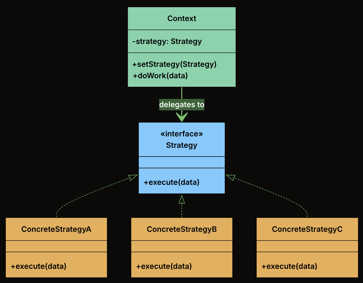
Strategy Interface: Declares the interface common to all supported algorithms. The Context uses this interface to call the algorithm defined by a ConcreteStrategy.
Concrete Strategies: Implements the algorithm using the Strategy interface. Each concrete strategy encapsulates a specific algorithm.
Context Class: This is the main class that uses a strategy to perform a task. It holds a reference to a Strategy object and delegates the calculation to it. The context doesn’t know or care which specific strategy is being used. It just knows that it has a strategy that can calculate a shipping cost.

🛠 Implementation

Define the Strategy Interface

interface ShippingStrategy {
    double calculateCost(Order order);
}

Implement Concrete Strategies

FlatRateShipping

class FlatRateShipping implements ShippingStrategy {
    private double rate;

    public FlatRateShipping(double rate) {
        this.rate = rate;
    }

    @Override
    public double calculateCost(Order order) {
        System.out.println("Calculating with Flat Rate strategy ($" + rate + ")");
        return rate;
    }
}

WeightBasedShipping

class WeightBasedShipping implements ShippingStrategy {
    private final double ratePerKg;

    public WeightBasedShipping(double ratePerKg) {
        this.ratePerKg = ratePerKg;
    }

    @Override
    public double calculateCost(Order order) {
        System.out.println("Calculating with Weight-Based strategy ($" + ratePerKg + "/kg)");
        return order.getTotalWeight() * ratePerKg;
    }
}

DistanceBasedShipping

class DistanceBasedShipping implements ShippingStrategy {
    private double ratePerKm;

    public DistanceBasedShipping(double ratePerKm) {
        this.ratePerKm = ratePerKm;
    }

    @Override
    public double calculateCost(Order order) {
        System.out.println("Calculating with Distance-Based strategy for zone: " + order.getDestinationZone());
        return switch (order.getDestinationZone()) {
            case "ZoneA" -> ratePerKm * 5.0;
            case "ZoneB" -> ratePerKm * 7.0;
            default -> ratePerKm * 10.0;
        };
    }
}

ThirdPartyApiShipping

class ThirdPartyApiShipping implements ShippingStrategy {
    private final double baseFee;
    private final double percentageFee;

    public ThirdPartyApiShipping(double baseFee, double percentageFee) {
        this.baseFee = baseFee;
        this.percentageFee = percentageFee;
    }

    @Override
    public double calculateCost(Order order) {
        System.out.println("Calculating with Third-Party API strategy.");
        // Simulate API call
        return baseFee + (order.getOrderValue() * percentageFee);
    }
}

Create the Context Class

class ShippingCostService {
    private ShippingStrategy strategy;

    // Constructor to set initial strategy
    public ShippingCostService(ShippingStrategy strategy) {
        this.strategy = strategy;
    }

    // Method to change strategy at runtime
    public void setStrategy(ShippingStrategy strategy) {
        System.out.println("ShippingCostService: Strategy changed to " + strategy.getClass().getSimpleName());
        this.strategy = strategy;
    }

    public double calculateShippingCost(Order order) {
        if (strategy == null) {
            throw new IllegalStateException("Shipping strategy not set.");
        }
        double cost = strategy.calculateCost(order);
        System.out.println("ShippingCostService: Final Calculated Shipping Cost: $" + cost +
                           " (using " + strategy.getClass().getSimpleName() + ")");
        return cost;
    }
}

Client Code

public class ECommerceAppV2 {
    public static void main(String[] args) {
        Order order1 = new Order();

        // Create different strategy instances
        ShippingStrategy flatRate = new FlatRateShipping(10.0);
        ShippingStrategy weightBased = new WeightBasedShipping(2.5);
        ShippingStrategy distanceBased = new DistanceBasedShipping(5.0);
        ShippingStrategy thirdParty = new ThirdPartyApiShipping(7.5, 0.02);

        // Create context with an initial strategy
        ShippingCostService shippingService = new ShippingCostService(flatRate);

        System.out.println("--- Order 1: Using Flat Rate (initial) ---");
        shippingService.calculateShippingCost(order1);

        System.out.println("\n--- Order 1: Changing to Weight-Based ---");
        shippingService.setStrategy(weightBased);
        shippingService.calculateShippingCost(order1);

        System.out.println("\n--- Order 1: Changing to Distance-Based ---");
        shippingService.setStrategy(distanceBased);
        shippingService.calculateShippingCost(order1);

        System.out.println("\n--- Order 1: Changing to Third-Party API ---");
        shippingService.setStrategy(thirdParty);
        shippingService.calculateShippingCost(order1);

        // Adding a NEW strategy is easy:
        // 1. Create a new class implementing ShippingStrategy (e.g., FreeShippingStrategy)
        // 2. Client can then instantiate and use it:
        //    ShippingStrategy freeShipping = new FreeShippingStrategy();
        //    shippingService.setStrategy(freeShipping);
        //    shippingService.calculateShippingCost(primeMemberOrder);
        // No modification to ShippingCostService is needed!
    }
}

Define the Strategy Interface

from abc import ABC, abstractmethod

class ShippingStrategy(ABC):
    @abstractmethod
    def calculate_cost(self, order) -> float:
        pass

Implement Concrete Strategies

FlatRateShipping

class FlatRateShipping(ShippingStrategy):
    def __init__(self, rate):
        self.rate = rate

    def calculate_cost(self, order):
        print(f"Calculating with Flat Rate strategy (${self.rate})")
        return self.rate

WeightBasedShipping

class WeightBasedShipping(ShippingStrategy):
    def __init__(self, rate_per_kg):
        self.rate_per_kg = rate_per_kg

    def calculate_cost(self, order):
        print(f"Calculating with Weight-Based strategy (${self.rate_per_kg}/kg)")
        return order.get_total_weight() * self.rate_per_kg

DistanceBasedShipping

class DistanceBasedShipping(ShippingStrategy):
    def __init__(self, rate_per_km):
        self.rate_per_km = rate_per_km

    def calculate_cost(self, order):
        print(f"Calculating with Distance-Based strategy for zone: {order.get_destination_zone()}")
        zone_mapping = {
            "ZoneA": self.rate_per_km * 5.0,
            "ZoneB": self.rate_per_km * 7.0
        }
        return zone_mapping.get(order.get_destination_zone(), self.rate_per_km * 10.0)

ThirdPartyApiShipping

class ThirdPartyApiShipping(ShippingStrategy):
    def __init__(self, base_fee, percentage_fee):
        self.base_fee = base_fee
        self.percentage_fee = percentage_fee

    def calculate_cost(self, order):
        print("Calculating with Third-Party API strategy.")
        # Simulate API call
        return self.base_fee + (order.get_order_value() * self.percentage_fee)

Create the Context Class

class ShippingCostService:
    def __init__(self, strategy):
        self.strategy = strategy

    def set_strategy(self, strategy):
        print(f"ShippingCostService: Strategy changed to {strategy.__class__.__name__}")
        self.strategy = strategy

    def calculate_shipping_cost(self, order):
        if self.strategy is None:
            raise ValueError("Shipping strategy not set.")

        cost = self.strategy.calculate_cost(order)
        print(f"ShippingCostService: Final Calculated Shipping Cost: ${cost} "
              f"(using {self.strategy.__class__.__name__})")
        return cost

Client Code

def ecommerce_app_v2():
    order1 = Order()

    # Create different strategy instances
    flat_rate = FlatRateShipping(10.0)
    weight_based = WeightBasedShipping(2.5)
    distance_based = DistanceBasedShipping(5.0)
    third_party = ThirdPartyApiShipping(7.5, 0.02)

    # Create context with an initial strategy
    shipping_service = ShippingCostService(flat_rate)

    print("--- Order 1: Using Flat Rate (initial) ---")
    shipping_service.calculate_shipping_cost(order1)

    print("\n--- Order 1: Changing to Weight-Based ---")
    shipping_service.set_strategy(weight_based)
    shipping_service.calculate_shipping_cost(order1)

    print("\n--- Order 1: Changing to Distance-Based ---")
    shipping_service.set_strategy(distance_based)
    shipping_service.calculate_shipping_cost(order1)

    print("\n--- Order 1: Changing to Third-Party API ---")
    shipping_service.set_strategy(third_party)
    shipping_service.calculate_shipping_cost(order1)

    # Adding a NEW strategy is easy:
    # 1. Create a new class implementing ShippingStrategy (e.g., FreeShippingStrategy)
    # 2. Client can then instantiate and use it:
    #    free_shipping = FreeShippingStrategy()
    #    shipping_service.set_strategy(free_shipping)
    #    shipping_service.calculate_shipping_cost(prime_member_order)
    # No modification to ShippingCostService is needed!

# Example usage
if __name__ == "__main__":
    ecommerce_app_v2()

Define the Strategy Interface

class ShippingStrategy {
public:
    virtual ~ShippingStrategy() {}
    virtual double calculateCost(const Order& order) = 0;
};

Implement Concrete Strategies

FlatRateShipping

class FlatRateShipping : public ShippingStrategy {
private:
    double rate;

public:
    FlatRateShipping(double r) : rate(r) {}

    double calculateCost(const Order& order) override {
        cout << "Calculating with Flat Rate strategy ($" << rate << ")" << endl;
        return rate;
    }
};

WeightBasedShipping

class WeightBasedShipping : public ShippingStrategy {
private:
    double ratePerKg;

public:
    WeightBasedShipping(double rateKg) : ratePerKg(rateKg) {}

    double calculateCost(const Order& order) override {
        cout << "Calculating with Weight-Based strategy ($" << ratePerKg << "/kg)" << endl;
        return order.getTotalWeight() * ratePerKg;
    }
};

DistanceBasedShipping

class DistanceBasedShipping : public ShippingStrategy {
private:
    double ratePerKm;

public:
    DistanceBasedShipping(double rateKm) : ratePerKm(rateKm) {}

    double calculateCost(const Order& order) override {
        cout << "Calculating with Distance-Based strategy for zone: " << order.getDestinationZone() << endl;

        if (order.getDestinationZone() == "ZoneA") {
            return ratePerKm * 5.0;
        } else if (order.getDestinationZone() == "ZoneB") {
            return ratePerKm * 7.0;
        } else {
            return ratePerKm * 10.0;
        }
    }
};

ThirdPartyApiShipping

class ThirdPartyApiShipping : public ShippingStrategy {
private:
    double baseFee;
    double percentageFee;

public:
    ThirdPartyApiShipping(double base, double percentage)
        : baseFee(base), percentageFee(percentage) {}

    double calculateCost(const Order& order) override {
        cout << "Calculating with Third-Party API strategy." << endl;
        // Simulate API call
        return baseFee + (order.getOrderValue() * percentageFee);
    }
};

Create the Context Class

class ShippingCostService {
private:
    ShippingStrategy* strategy;

public:
    ShippingCostService(ShippingStrategy* s) : strategy(s) {}

    void setStrategy(ShippingStrategy* s) {
        cout << "ShippingCostService: Strategy changed" << endl;
        strategy = s;
    }

    double calculateShippingCost(const Order& order) {
        if (strategy == nullptr) {
            throw invalid_argument("Shipping strategy not set.");
        }

        double cost = strategy->calculateCost(order);
        cout << "ShippingCostService: Final Calculated Shipping Cost: $" << cost << endl;
        return cost;
    }
};

Client Code

void ecommerceAppV2() {
    Order order1;

    // Create different strategy instances
    FlatRateShipping flatRate(10.0);
    WeightBasedShipping weightBased(2.5);
    DistanceBasedShipping distanceBased(5.0);
    ThirdPartyApiShipping thirdParty(7.5, 0.02);

    // Create context with an initial strategy
    ShippingCostService shippingService(&flatRate);

    cout << "--- Order 1: Using Flat Rate (initial) ---" << endl;
    shippingService.calculateShippingCost(order1);

    cout << "\n--- Order 1: Changing to Weight-Based ---" << endl;
    shippingService.setStrategy(&weightBased);
    shippingService.calculateShippingCost(order1);

    cout << "\n--- Order 1: Changing to Distance-Based ---" << endl;
    shippingService.setStrategy(&distanceBased);
    shippingService.calculateShippingCost(order1);

    cout << "\n--- Order 1: Changing to Third-Party API ---" << endl;
    shippingService.setStrategy(&thirdParty);
    shippingService.calculateShippingCost(order1);

    // Adding a NEW strategy is easy:
    // 1. Create a new class implementing ShippingStrategy (e.g., FreeShippingStrategy)
    // 2. Client can then instantiate and use it:
    //    FreeShippingStrategy freeShipping;
    //    shippingService.setStrategy(&freeShipping);
    //    shippingService.calculateShippingCost(primeMemberOrder);
    // No modification to ShippingCostService is needed!
}

int main() {
    cout << "\n\n=== Strategy Pattern Approach ===" << endl;
    ecommerceAppV2();
    return 0;
}

Define the Strategy Interface

interface IShippingStrategy
{
    double CalculateCost(Order order);
}

Implement Concrete Strategies

FlatRateShipping

class FlatRateShipping : IShippingStrategy
{
    private double rate;

    public FlatRateShipping(double rate)
    {
        this.rate = rate;
    }

    public double CalculateCost(Order order)
    {
        Console.WriteLine($"Calculating with Flat Rate strategy (${rate})");
        return rate;
    }
}

WeightBasedShipping

class WeightBasedShipping : IShippingStrategy
{
    private double ratePerKg;

    public WeightBasedShipping(double ratePerKg)
    {
        this.ratePerKg = ratePerKg;
    }

    public double CalculateCost(Order order)
    {
        Console.WriteLine($"Calculating with Weight-Based strategy (${ratePerKg}/kg)");
        return order.GetTotalWeight() * ratePerKg;
    }
}

DistanceBasedShipping

class DistanceBasedShipping : IShippingStrategy
{
    private double ratePerKm;

    public DistanceBasedShipping(double ratePerKm)
    {
        this.ratePerKm = ratePerKm;
    }

    public double CalculateCost(Order order)
    {
        Console.WriteLine($"Calculating with Distance-Based strategy for zone: {order.GetDestinationZone()}");

        switch (order.GetDestinationZone())
        {
            case "ZoneA":
                return ratePerKm * 5.0;
            case "ZoneB":
                return ratePerKm * 7.0;
            default:
                return ratePerKm * 10.0;
        }
    }
}

ThirdPartyApiShipping

class ThirdPartyApiShipping : IShippingStrategy
{
    private double baseFee;
    private double percentageFee;

    public ThirdPartyApiShipping(double baseFee, double percentageFee)
    {
        this.baseFee = baseFee;
        this.percentageFee = percentageFee;
    }

    public double CalculateCost(Order order)
    {
        Console.WriteLine("Calculating with Third-Party API strategy.");
        // Simulate API call
        return baseFee + (order.GetOrderValue() * percentageFee);
    }
}

Create the Context Class

class ShippingCostService
{
    private IShippingStrategy strategy;

    public ShippingCostService(IShippingStrategy strategy)
    {
        this.strategy = strategy;
    }

    public void SetStrategy(IShippingStrategy strategy)
    {
        Console.WriteLine($"ShippingCostService: Strategy changed to {strategy.GetType().Name}");
        this.strategy = strategy;
    }

    public double CalculateShippingCost(Order order)
    {
        if (strategy == null)
        {
            throw new InvalidOperationException("Shipping strategy not set.");
        }

        double cost = strategy.CalculateCost(order);
        Console.WriteLine($"ShippingCostService: Final Calculated Shipping Cost: ${cost} " +
                         $"(using {strategy.GetType().Name})");
        return cost;
    }
}

Client Code

public class Program
{
    public static void ECommerceAppV2()
    {
        Order order1 = new Order();

        // Create different strategy instances
        IShippingStrategy flatRate = new FlatRateShipping(10.0);
        IShippingStrategy weightBased = new WeightBasedShipping(2.5);
        IShippingStrategy distanceBased = new DistanceBasedShipping(5.0);
        IShippingStrategy thirdParty = new ThirdPartyApiShipping(7.5, 0.02);

        // Create context with an initial strategy
        ShippingCostService shippingService = new ShippingCostService(flatRate);

        Console.WriteLine("--- Order 1: Using Flat Rate (initial) ---");
        shippingService.CalculateShippingCost(order1);

        Console.WriteLine("\n--- Order 1: Changing to Weight-Based ---");
        shippingService.SetStrategy(weightBased);
        shippingService.CalculateShippingCost(order1);

        Console.WriteLine("\n--- Order 1: Changing to Distance-Based ---");
        shippingService.SetStrategy(distanceBased);
        shippingService.CalculateShippingCost(order1);

        Console.WriteLine("\n--- Order 1: Changing to Third-Party API ---");
        shippingService.SetStrategy(thirdParty);
        shippingService.CalculateShippingCost(order1);

        // Adding a NEW strategy is easy:
        // 1. Create a new class implementing IShippingStrategy (e.g., FreeShippingStrategy)
        // 2. Client can then instantiate and use it:
        //    IShippingStrategy freeShipping = new FreeShippingStrategy();
        //    shippingService.SetStrategy(freeShipping);
        //    shippingService.CalculateShippingCost(primeMemberOrder);
        // No modification to ShippingCostService is needed!
    }

    public static void Main(string[] args)
    {
        Console.WriteLine("\n\n=== Strategy Pattern Approach ===");
        ECommerceAppV2();
    }
}

Define the Strategy Interface

interface ShippingStrategy {
  calculateCost(order: Order): number;
}

Implement Concrete Strategies

FlatRateShipping

class FlatRateShipping implements ShippingStrategy {
  private rate: number;

  constructor(rate: number) {
    this.rate = rate;
  }

  calculateCost(order: Order): number {
    console.log("Calculating with Flat Rate strategy ($" + this.rate + ")");
    return this.rate;
  }
}

WeightBasedShipping

class WeightBasedShipping implements ShippingStrategy {
  private readonly ratePerKg: number;

  constructor(ratePerKg: number) {
    this.ratePerKg = ratePerKg;
  }

  calculateCost(order: Order): number {
    console.log(
      "Calculating with Weight-Based strategy ($" + this.ratePerKg + "/kg)",
    );
    return order.getTotalWeight() * this.ratePerKg;
  }
}

DistanceBasedShipping

class DistanceBasedShipping implements ShippingStrategy {
  private ratePerKm: number;

  constructor(ratePerKm: number) {
    this.ratePerKm = ratePerKm;
  }

  calculateCost(order: Order): number {
    console.log(
      "Calculating with Distance-Based strategy for zone: " +
        order.getDestinationZone(),
    );
    switch (order.getDestinationZone()) {
      case "ZoneA":
        return this.ratePerKm * 5.0;
      case "ZoneB":
        return this.ratePerKm * 7.0;
      default:
        return this.ratePerKm * 10.0;
    }
  }
}

ThirdPartyApiShipping

class ThirdPartyApiShipping implements ShippingStrategy {
  private readonly baseFee: number;
  private readonly percentageFee: number;

  constructor(baseFee: number, percentageFee: number) {
    this.baseFee = baseFee;
    this.percentageFee = percentageFee;
  }

  calculateCost(order: Order): number {
    console.log("Calculating with Third-Party API strategy.");
    // Simulate API call
    return this.baseFee + order.getOrderValue() * this.percentageFee;
  }
}

Create the Context Class

class ShippingCostService {
  private strategy: ShippingStrategy;

  // Constructor to set initial strategy
  constructor(strategy: ShippingStrategy) {
    this.strategy = strategy;
  }

  // Method to change strategy at runtime
  setStrategy(strategy: ShippingStrategy): void {
    console.log(
      "ShippingCostService: Strategy changed to " + strategy.constructor.name,
    );
    this.strategy = strategy;
  }

  calculateShippingCost(order: Order): number {
    if (!this.strategy) {
      throw new Error("Shipping strategy not set.");
    }
    const cost = this.strategy.calculateCost(order);
    console.log(
      "ShippingCostService: Final Calculated Shipping Cost: $" +
        cost +
        " (using " +
        this.strategy.constructor.name +
        ")",
    );
    return cost;
  }
}

Client Code

class ECommerceAppV2 {
  static main(): void {
    const order1 = new Order();

    // Create different strategy instances
    const flatRate: ShippingStrategy = new FlatRateShipping(10.0);
    const weightBased: ShippingStrategy = new WeightBasedShipping(2.5);
    const distanceBased: ShippingStrategy = new DistanceBasedShipping(5.0);
    const thirdParty: ShippingStrategy = new ThirdPartyApiShipping(7.5, 0.02);

    // Create context with an initial strategy
    const shippingService = new ShippingCostService(flatRate);

    console.log("--- Order 1: Using Flat Rate (initial) ---");
    shippingService.calculateShippingCost(order1);

    console.log("\n--- Order 1: Changing to Weight-Based ---");
    shippingService.setStrategy(weightBased);
    shippingService.calculateShippingCost(order1);

    console.log("\n--- Order 1: Changing to Distance-Based ---");
    shippingService.setStrategy(distanceBased);
    shippingService.calculateShippingCost(order1);

    console.log("\n--- Order 1: Changing to Third-Party API ---");
    shippingService.setStrategy(thirdParty);
    shippingService.calculateShippingCost(order1);

    // Adding a NEW strategy is easy:
    // 1. Create a new class implementing ShippingStrategy (e.g., FreeShippingStrategy)
    // 2. Client can then instantiate and use it:
    //    const freeShipping: ShippingStrategy = new FreeShippingStrategy();
    //    shippingService.setStrategy(freeShipping);
    //    shippingService.calculateShippingCost(primeMemberOrder);
    // No modification to ShippingCostService is needed!
  }
}

Observer

📖 Definition

The Observer Design Pattern is a behavioral pattern that defines a one-to-many dependency between objects so that when one object (the subject) changes its state, all its dependents (observers) are automatically notified and updated.

This pattern shines in scenarios where:

You have multiple parts of the system that need to react to a change in one central component.
You want to decouple the publisher of data from the subscribers who react to it.
You need a dynamic, event-driven communication model without hardcoding who is listening to whom.

🧩 Class Diagram

Observer Pattern Class Diagram

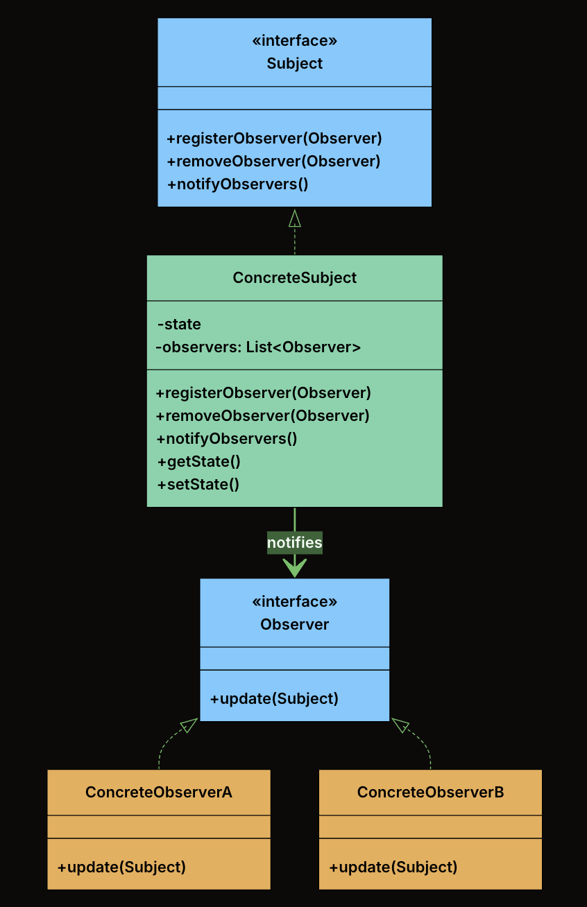
Subject Interface: Declares the interface for managing observers, registering, removing, and notifying them. Defines registerObserver(), removeObserver(), and notifyObservers() methods. The subject holds a list of observers typed to the Observer interface, not to concrete classes. This means any class that implements the Observer interface can register, and the subject never needs to know what it is.
Observer Interface: Declares the update() method that the subject calls when its state changes. All modules that want to listen to fitness data changes will implement this interface.
ConcreteSubject: Implements the Subject interface. Holds the actual state and notifies observers when that state changes. Maintain a list of registered observers and calls notifyObservers() whenever its state changes.
ConcreteObservers: Implements the Observer interface. Defines what happens when the subject’s state changes. When update() is called, each observer pulls relevant data from the subject and performs its own logic (e.g., update UI, log progress, send alerts).

🛠 Implementation

Define the Observer Interface

interface FitnessDataObserver {
    void update(FitnessData data);
}

Define the Subject Interface

interface FitnessDataSubject {
    void registerObserver(FitnessDataObserver observer);
    void removeObserver(FitnessDataObserver observer);
    void notifyObservers();
}

Implement the ConcreteSubject

public class FitnessData implements FitnessDataSubject {
    private int steps;
    private int activeMinutes;
    private int calories;

    private final List<FitnessDataObserver> observers = new ArrayList<>();

    @Override
    public void registerObserver(FitnessDataObserver observer) {
        observers.add(observer);
    }

    @Override
    public void removeObserver(FitnessDataObserver observer) {
        observers.remove(observer);
    }

    @Override
    public void notifyObservers() {
        for (FitnessDataObserver observer : observers) {
            observer.update(this);
        }
    }

    public void newFitnessDataPushed(int steps, int activeMinutes, int calories) {
        this.steps = steps;
        this.activeMinutes = activeMinutes;
        this.calories = calories;

        System.out.println("\nFitnessData: New data received – Steps: " + steps +
            ", Active Minutes: " + activeMinutes + ", Calories: " + calories);

        notifyObservers();
    }

    public void dailyReset() {
        this.steps = 0;
        this.activeMinutes = 0;
        this.calories = 0;

        System.out.println("\nFitnessData: Daily reset performed.");
        notifyObservers();
    }

    // Getters
    public int getSteps() { return steps; }
    public int getActiveMinutes() { return activeMinutes; }
    public int getCalories() { return calories; }
}

Implement Concrete Observers

LiveActivityDisplay

class LiveActivityDisplay implements FitnessDataObserver {
    @Override
    public void update(FitnessData data) {
        System.out.println("Live Display → Steps: " + data.getSteps() +
            " | Active Minutes: " + data.getActiveMinutes() +
            " | Calories: " + data.getCalories());
    }
}

ProgressLogger

class ProgressLogger implements FitnessDataObserver {
    @Override
    public void update(FitnessData data) {
        System.out.println("Logger → Saving to DB: Steps=" + data.getSteps() +
            ", ActiveMinutes=" + data.getActiveMinutes() +
            ", Calories=" + data.getCalories());
        // Simulated DB/file write...
    }
}

GoalNotifier

class GoalNotifier implements FitnessDataObserver {
    private final int stepGoal = 10000;
    private boolean goalReached = false;

    @Override
    public void update(FitnessData data) {
        if (data.getSteps() >= stepGoal && !goalReached) {
            System.out.println("Notifier → 🎉 Goal Reached! You've hit " + stepGoal + " steps!");
            goalReached = true;
        }
    }

    public void reset() {
        goalReached = false;
    }
}

Client Code

public class FitnessAppObserverDemo {
    public static void main(String[] args) {
        FitnessData fitnessData = new FitnessData();

        LiveActivityDisplay display = new LiveActivityDisplay();
        ProgressLogger logger = new ProgressLogger();
        GoalNotifier notifier = new GoalNotifier();

        // Register observers
        fitnessData.registerObserver(display);
        fitnessData.registerObserver(logger);
        fitnessData.registerObserver(notifier);

        // Simulate updates
        fitnessData.newFitnessDataPushed(500, 5, 20);
        fitnessData.newFitnessDataPushed(9800, 85, 350);
        fitnessData.newFitnessDataPushed(10100, 90, 380);

        // Remove logger and reset notifier
        fitnessData.removeObserver(logger);
        notifier.reset();
        fitnessData.dailyReset();
    }
}

Define the Observer Interface

from abc import ABC, abstractmethod

class FitnessDataObserver(ABC):
    @abstractmethod
    def update(self, data):
        pass

Define the Subject Interface

class FitnessDataSubject(ABC):
    @abstractmethod
    def register_observer(self, observer):
        pass

    @abstractmethod
    def remove_observer(self, observer):
        pass

    @abstractmethod
    def notify_observers(self):
        pass

Implement the ConcreteSubject

class FitnessData(FitnessDataSubject):
    def __init__(self):
        self.steps = 0
        self.active_minutes = 0
        self.calories = 0
        self.observers = []

    def register_observer(self, observer):
        self.observers.append(observer)

    def remove_observer(self, observer):
        if observer in self.observers:
            self.observers.remove(observer)

    def notify_observers(self):
        for observer in self.observers:
            observer.update(self)

    def new_fitness_data_pushed(self, steps, active_minutes, calories):
        self.steps = steps
        self.active_minutes = active_minutes
        self.calories = calories

        print(f"\nFitnessData: New data received – Steps: {steps}, "
              f"Active Minutes: {active_minutes}, Calories: {calories}")

        self.notify_observers()

    def daily_reset(self):
        self.steps = 0
        self.active_minutes = 0
        self.calories = 0

        print("\nFitnessData: Daily reset performed.")
        self.notify_observers()

    # Getters
    def get_steps(self):
        return self.steps

    def get_active_minutes(self):
        return self.active_minutes

    def get_calories(self):
        return self.calories

Implement Concrete Observers

LiveActivityDisplay

class LiveActivityDisplay(FitnessDataObserver):
    def update(self, data):
        print(f"Live Display → Steps: {data.get_steps()} "
              f"| Active Minutes: {data.get_active_minutes()} "
              f"| Calories: {data.get_calories()}")

ProgressLogger

class ProgressLogger(FitnessDataObserver):
    def update(self, data):
        print(f"Logger → Saving to DB: Steps={data.get_steps()}, "
              f"ActiveMinutes={data.get_active_minutes()}, "
              f"Calories={data.get_calories()}")
        # Simulated DB/file write...

GoalNotifier

class GoalNotifier(FitnessDataObserver):
    def __init__(self):
        self.step_goal = 10000
        self.goal_reached = False

    def update(self, data):
        if data.get_steps() >= self.step_goal and not self.goal_reached:
            print(f"Notifier → 🎉 Goal Reached! You've hit {self.step_goal} steps!")
            self.goal_reached = True

    def reset(self):
        self.goal_reached = False

Client Code

def fitness_app_observer_demo():
    fitness_data = FitnessData()

    display = LiveActivityDisplay()
    logger = ProgressLogger()
    notifier = GoalNotifier()

    # Register observers
    fitness_data.register_observer(display)
    fitness_data.register_observer(logger)
    fitness_data.register_observer(notifier)

    # Simulate updates
    fitness_data.new_fitness_data_pushed(500, 5, 20)
    fitness_data.new_fitness_data_pushed(9800, 85, 350)
    fitness_data.new_fitness_data_pushed(10100, 90, 380)

    # Remove logger and reset notifier
    fitness_data.remove_observer(logger)
    notifier.reset()
    fitness_data.daily_reset()

if __name__ == "__main__":
    print("=== Observer Pattern Approach ===")
    fitness_app_observer_demo()

Define the Observer Interface

class FitnessDataObserver {
public:
    virtual ~FitnessDataObserver() {}
    virtual void update(FitnessData* data) = 0;
};

Define the Subject Interface

class FitnessDataSubject {
public:
    virtual ~FitnessDataSubject() {}
    virtual void registerObserver(FitnessDataObserver* observer) = 0;
    virtual void removeObserver(FitnessDataObserver* observer) = 0;
    virtual void notifyObservers() = 0;
};

Implement the ConcreteSubject

class FitnessData : public FitnessDataSubject {
private:
    int steps;
    int activeMinutes;
    int calories;
    vector<FitnessDataObserver*> observers;

public:
    FitnessData() : steps(0), activeMinutes(0), calories(0) {}

    void registerObserver(FitnessDataObserver* observer) override {
        observers.push_back(observer);
    }

    void removeObserver(FitnessDataObserver* observer) override {
        observers.erase(remove(observers.begin(), observers.end(), observer), observers.end());
    }

    void notifyObservers() override {
        for (FitnessDataObserver* observer : observers) {
            observer->update(this);
        }
    }

    void newFitnessDataPushed(int newSteps, int newActiveMinutes, int newCalories) {
        steps = newSteps;
        activeMinutes = newActiveMinutes;
        calories = newCalories;

        cout << "\nFitnessData: New data received – Steps: " << steps
             << ", Active Minutes: " << activeMinutes << ", Calories: " << calories << endl;

        notifyObservers();
    }

    void dailyReset() {
        steps = 0;
        activeMinutes = 0;
        calories = 0;

        cout << "\nFitnessData: Daily reset performed." << endl;
        notifyObservers();
    }

    // Getters
    int getSteps() const { return steps; }
    int getActiveMinutes() const { return activeMinutes; }
    int getCalories() const { return calories; }
};

Implement Concrete Observers

LiveActivityDisplay

class LiveActivityDisplay : public FitnessDataObserver {
public:
    void update(FitnessData* data) override {
        cout << "Live Display → Steps: " << data->getSteps()
             << " | Active Minutes: " << data->getActiveMinutes()
             << " | Calories: " << data->getCalories() << endl;
    }
};

ProgressLogger

class ProgressLogger : public FitnessDataObserver {
public:
    void update(FitnessData* data) override {
        cout << "Logger → Saving to DB: Steps=" << data->getSteps()
             << ", ActiveMinutes=" << data->getActiveMinutes()
             << ", Calories=" << data->getCalories() << endl;
        // Simulated DB/file write...
    }
};

GoalNotifier

class GoalNotifier : public FitnessDataObserver {
private:
    int stepGoal;
    bool goalReached;

public:
    GoalNotifier() : stepGoal(10000), goalReached(false) {}

    void update(FitnessData* data) override {
        if (data->getSteps() >= stepGoal && !goalReached) {
            cout << "Notifier → 🎉 Goal Reached! You've hit " << stepGoal << " steps!" << endl;
            goalReached = true;
        }
    }

    void reset() {
        goalReached = false;
    }
};

Client Code

int main() {
    cout << "=== Observer Pattern Approach ===" << endl;

    FitnessData fitnessData;

    LiveActivityDisplay display;
    ProgressLogger logger;
    GoalNotifier notifier;

    // Register observers
    fitnessData.registerObserver(&display);
    fitnessData.registerObserver(&logger);
    fitnessData.registerObserver(&notifier);

    // Simulate updates
    fitnessData.newFitnessDataPushed(500, 5, 20);
    fitnessData.newFitnessDataPushed(9800, 85, 350);
    fitnessData.newFitnessDataPushed(10100, 90, 380);

    // Remove logger and reset notifier
    fitnessData.removeObserver(&logger);
    notifier.reset();
    fitnessData.dailyReset();

    return 0;
}

Define the Observer Interface

interface IFitnessDataObserver
{
    void Update(FitnessData data);
}

Define the Subject Interface

interface IFitnessDataSubject
{
    void RegisterObserver(IFitnessDataObserver observer);
    void RemoveObserver(IFitnessDataObserver observer);
    void NotifyObservers();
}

Implement the ConcreteSubject

class FitnessData : IFitnessDataSubject
{
    private int steps;
    private int activeMinutes;
    private int calories;
    private List<IFitnessDataObserver> observers = new List<IFitnessDataObserver>();

    public void RegisterObserver(IFitnessDataObserver observer)
    {
        observers.Add(observer);
    }

    public void RemoveObserver(IFitnessDataObserver observer)
    {
        observers.Remove(observer);
    }

    public void NotifyObservers()
    {
        foreach (IFitnessDataObserver observer in observers)
        {
            observer.Update(this);
        }
    }

    public void NewFitnessDataPushed(int newSteps, int newActiveMinutes, int newCalories)
    {
        steps = newSteps;
        activeMinutes = newActiveMinutes;
        calories = newCalories;

        Console.WriteLine($"\nFitnessData: New data received – Steps: {steps}, Active Minutes: {activeMinutes}, Calories: {calories}");

        NotifyObservers();
    }

    public void DailyReset()
    {
        steps = 0;
        activeMinutes = 0;
        calories = 0;

        Console.WriteLine("\nFitnessData: Daily reset performed.");
        NotifyObservers();
    }

    // Getters
    public int GetSteps() { return steps; }
    public int GetActiveMinutes() { return activeMinutes; }
    public int GetCalories() { return calories; }
}

Implement Concrete Observers

LiveActivityDisplay

class LiveActivityDisplay : IFitnessDataObserver
{
    public void Update(FitnessData data)
    {
        Console.WriteLine($"Live Display → Steps: {data.GetSteps()} | Active Minutes: {data.GetActiveMinutes()} | Calories: {data.GetCalories()}");
    }
}

ProgressLogger

class ProgressLogger : IFitnessDataObserver
{
    public void Update(FitnessData data)
    {
        Console.WriteLine($"Logger → Saving to DB: Steps={data.GetSteps()}, ActiveMinutes={data.GetActiveMinutes()}, Calories={data.GetCalories()}");
        // Simulated DB/file write...
    }
}

GoalNotifier

class GoalNotifier : IFitnessDataObserver
{
    private int stepGoal = 10000;
    private bool goalReached = false;

    public void Update(FitnessData data)
    {
        if (data.GetSteps() >= stepGoal && !goalReached)
        {
            Console.WriteLine($"Notifier → 🎉 Goal Reached! You've hit {stepGoal} steps!");
            goalReached = true;
        }
    }

    public void Reset()
    {
        goalReached = false;
    }
}

Client Code

public class Program
{
    public static void Main(string[] args)
    {
        Console.WriteLine("=== Observer Pattern Approach ===");

        FitnessData fitnessData = new FitnessData();

        LiveActivityDisplay display = new LiveActivityDisplay();
        ProgressLogger logger = new ProgressLogger();
        GoalNotifier notifier = new GoalNotifier();

        // Register observers
        fitnessData.RegisterObserver(display);
        fitnessData.RegisterObserver(logger);
        fitnessData.RegisterObserver(notifier);

        // Simulate updates
        fitnessData.NewFitnessDataPushed(500, 5, 20);
        fitnessData.NewFitnessDataPushed(9800, 85, 350);
        fitnessData.NewFitnessDataPushed(10100, 90, 380);

        // Remove logger and reset notifier
        fitnessData.RemoveObserver(logger);
        notifier.Reset();
        fitnessData.DailyReset();
    }
}

Define the Observer Interface

interface FitnessDataObserver {
  update(data: FitnessData): void;
}

Define the Subject Interface

interface FitnessDataSubject {
  registerObserver(observer: FitnessDataObserver): void;
  removeObserver(observer: FitnessDataObserver): void;
  notifyObservers(): void;
}

Implement the ConcreteSubject

class FitnessData implements FitnessDataSubject {
  private steps: number;
  private activeMinutes: number;
  private calories: number;

  private readonly observers: FitnessDataObserver[] = [];

  registerObserver(observer: FitnessDataObserver): void {
    this.observers.push(observer);
  }

  removeObserver(observer: FitnessDataObserver): void {
    const index = this.observers.indexOf(observer);
    if (index > -1) {
      this.observers.splice(index, 1);
    }
  }

  notifyObservers(): void {
    for (const observer of this.observers) {
      observer.update(this);
    }
  }

  newFitnessDataPushed(
    steps: number,
    activeMinutes: number,
    calories: number,
  ): void {
    this.steps = steps;
    this.activeMinutes = activeMinutes;
    this.calories = calories;

    console.log(
      "\nFitnessData: New data received – Steps: " +
        steps +
        ", Active Minutes: " +
        activeMinutes +
        ", Calories: " +
        calories,
    );

    this.notifyObservers();
  }

  dailyReset(): void {
    this.steps = 0;
    this.activeMinutes = 0;
    this.calories = 0;

    console.log("\nFitnessData: Daily reset performed.");
    this.notifyObservers();
  }

  // Getters
  getSteps(): number {
    return this.steps;
  }
  getActiveMinutes(): number {
    return this.activeMinutes;
  }
  getCalories(): number {
    return this.calories;
  }
}

Implement Concrete Observers

LiveActivityDisplay

class LiveActivityDisplay implements FitnessDataObserver {
  update(data: FitnessData): void {
    console.log(
      "Live Display → Steps: " +
        data.getSteps() +
        " | Active Minutes: " +
        data.getActiveMinutes() +
        " | Calories: " +
        data.getCalories(),
    );
  }
}

ProgressLogger

class ProgressLogger implements FitnessDataObserver {
  update(data: FitnessData): void {
    console.log(
      "Logger → Saving to DB: Steps=" +
        data.getSteps() +
        ", ActiveMinutes=" +
        data.getActiveMinutes() +
        ", Calories=" +
        data.getCalories(),
    );
    // Simulated DB/file write...
  }
}

GoalNotifier

class GoalNotifier implements FitnessDataObserver {
  private readonly stepGoal: number = 10000;
  private goalReached: boolean = false;

  update(data: FitnessData): void {
    if (data.getSteps() >= this.stepGoal && !this.goalReached) {
      console.log(
        "Notifier → 🎉 Goal Reached! You've hit " + this.stepGoal + " steps!",
      );
      this.goalReached = true;
    }
  }

  reset(): void {
    this.goalReached = false;
  }
}

Client Code

const fitnessData = new FitnessData();

const display = new LiveActivityDisplay();
const logger = new ProgressLogger();
const notifier = new GoalNotifier();

// Register observers
fitnessData.registerObserver(display);
fitnessData.registerObserver(logger);
fitnessData.registerObserver(notifier);

// Simulate updates
fitnessData.newFitnessDataPushed(500, 5, 20);
fitnessData.newFitnessDataPushed(9800, 85, 350);
fitnessData.newFitnessDataPushed(10100, 90, 380);

// Remove logger and reset notifier
fitnessData.removeObserver(logger);
notifier.reset();
fitnessData.dailyReset();

Design

146. LRU Cache
155. Min Stack
173. Binary Search Tree Iterator
208. Implement Trie (Prefix Tree)
211. Design Add and Search Words Data Structure
225. Implement Stack using Queues
232. Implement Queue using Stacks
284. Peeking Iterator
303. Range Sum Query - Immutable
304. Range Sum Query 2D - Immutable
307. Range Sum Query - Mutable
341. Flatten Nested List Iterator
355. Design Twitter
703. Kth Largest Element in a Stream
705. Design HashSet
706. Design HashMap
933. Number of Recent Calls
1603. Design Parking System
1656. Design an Ordered Stream
3242. Design Neighbor Sum Service

146. LRU Cache

LeetCode Link: LRU Cache
Difficulty: Medium
Topic(s): Design, Hash Table, Linked List
Company: Twitch

🧠 Problem Statement

Design a data structure that follows the constraints of a Least Recently Used (LRU) cache.

Implement the LRUCache class:

LRUCache(int capacity) Initialize the LRU cache with positive size capacity.
int get(int key) Return the value of the key if the key exists, otherwise return -1.
void put(int key, int value) Update the value of the key if the key exists. Otherwise, add the key-value pair to the cache. If the number of keys exceeds the capacity from this operation, evict the least recently used key.

The functions get and put must each run in O(1) average time complexity.

Example 1:

Input
["LRUCache", "put", "put", "get", "put", "get", "put", "get", "get", "get"]
[[2], [1, 1], [2, 2], [1], [3, 3], [2], [4, 4], [1], [3], [4]]

Output
[null, null, null, 1, null, -1, null, -1, 3, 4]

Explanation
LRUCache lRUCache = new LRUCache(2);
lRUCache.put(1, 1); // cache is {1=1}
lRUCache.put(2, 2); // cache is {1=1, 2=2}
lRUCache.get(1);    // return 1
lRUCache.put(3, 3); // LRU key was 2, evicts key 2, cache is {1=1, 3=3}
lRUCache.get(2);    // returns -1 (not found)
lRUCache.put(4, 4); // LRU key was 1, evicts key 1, cache is {4=4, 3=3}
lRUCache.get(1);    // return -1 (not found)
lRUCache.get(3);    // return 3
lRUCache.get(4);    // return 4

🧩 Approach

To implement an LRU Cache, we can use a combination of a hash map and a doubly linked list. The hash map will allow us to access the cache items in O(1) time, while the doubly linked list will help us maintain the order of usage of the cache items. The most recently used item will be at the end of the list, and the least recently used item will be at the beginning of the list. When we access an item, we will move it to the end of the list to mark it as most recently used. When we need to evict an item due to capacity constraints, we will remove the item at the beginning of the list, which is the least recently used item.

💡 Solution

from typing import Optional, Dict

class Node:

    def __init__(self, key: int, value: int):
        """Initializes a Node with the given key and value.

        Args:
            key (int): The key associated with the node.
            value (int): The value associated with the node.

        Returns:
            None
        """
        self.key: int = key
        self.value: int = value
        self.prev: Optional[Node] = None
        self.next: Optional[Node] = None

class LRUCache:

    def __init__(self, capacity: int):
        """Initializes the LRUCache object with the given capacity.

        Args:
            capacity (int): The maximum number of items that the cache can hold.

        Returns:
            None
        """
        self.__capacity: int = capacity
        self.__hashmap: Dict[int, Node] = {}
        self.__left: Node = Node(0, 0)
        self.__right: Node = Node(0, 0)
        self.__left.next = self.__right
        self.__right.prev = self.__left

    def __insert(self, node: Node) -> None:
        """Inserts a node at the end of the doubly linked list (right before the right dummy node).

        Args:
            node (Node): The node to be inserted into the list.

        Returns:
            None
        """
        prev: Node = self.__right.prev
        nxt: Node = self.__right
        prev.next = node
        nxt.prev = node
        node.prev = prev
        node.next = nxt

    def __remove(self, node: Node) -> None:
        """Removes a node from the doubly linked list.

        Args:
            node (Node): The node to be removed from the list.

        Returns:
            None
        """
        prev: Node = node.prev
        nxt: Node = node.next
        prev.next = nxt
        nxt.prev = prev

    def get(self, key: int) -> int:
        """Returns the value of the key if the key exists, otherwise returns -1.

        Args:
            key (int): The key to be accessed in the cache.

        Returns:
            int: The value associated with the key if it exists, otherwise -1.
        """
        if key in self.__hashmap:
            self.__remove(self.__hashmap[key])
            self.__insert(self.__hashmap[key])
            return self.__hashmap[key].value
        return -1

    def put(self, key: int, value: int) -> None:
        """Updates the value of the key if the key exists. Otherwise, adds the key-value pair to the cache. If the number of keys exceeds the capacity from this operation, evicts the least recently used key.

        Args:
            key (int): The key to be added or updated in the cache.
            value (int): The value to be associated with the key.

        Returns:
            None
        """
        if key in self.__hashmap:
            self.__remove(self.__hashmap[key])
        self.__hashmap[key] = Node(key, value)
        self.__insert(self.__hashmap[key])

        if len(self.__hashmap) > self.__capacity:
            lru: Node = self.__left.next
            self.__remove(lru)
            del self.__hashmap[lru.key]

🧮 Complexity Analysis

Time Complexity:
- get: O(1)
- put: O(1)
Space Complexity: O(n) where n is the capacity of the cache.

155. Min Stack

LeetCode Link: Min Stack
Difficulty: Easy
Topic(s): Design, Stack
Company: Amazon

🧠 Problem Statement

Design a stack that supports push, pop, top, and retrieving the minimum element in constant time.

Implement the MinStack class:

MinStack() initializes the stack object.

void push(int val) pushes the element val onto the stack.

void pop() removes the element on the top of the stack.

int top() gets the top element of the stack.

int getMin() retrieves the minimum element in the stack.

You must implement a solution with O(1) time complexity for each function.

Example 1:
Input
["MinStack","push","push","push","getMin","pop","top","getMin"]
[[],[-2],[0],[-3],[],[],[],[]]

Output
[null,null,null,null,-3,null,0,-2]

Explanation
MinStack minStack = new MinStack();
minStack.push(-2);
minStack.push(0);
minStack.push(-3);
minStack.getMin(); // return -3
minStack.pop();
minStack.top();    // return 0
minStack.getMin(); // return -2

🧩 Approach

To implement a stack that supports retrieving the minimum element in constant time, we can use two stacks. The first stack will be used to store all the elements of the stack, while the second stack will be used to keep track of the minimum elements. Whenever we push a new element onto the main stack, we compare it with the current minimum (the top of the minimum stack). If the new element is smaller than or equal to the current minimum, we also push it onto the minimum stack. When we pop an element from the main stack, if that element is the same as the current minimum, we also pop it from the minimum stack. This way, the top of the minimum stack will always represent the minimum element in the main stack.

💡 Solution

from typing import List

class MinStack:

    def __init__(self):
        self.__stack: List[int] = []
        self.__minStack: List[int] = []

    def push(self, val: int) -> None:
        """Pushes an element onto the stack and updates the minimum stack if necessary.

        Args:
            val (int): The value to be pushed onto the stack.

        Returns:
            None
        """
        self.__stack.append(val)
        val: int = min(val, self.__minStack[-1] if self.__minStack else val)
        self.__minStack.append(val)

    def pop(self) -> None:
        """Removes the element on the top of the stack and updates the minimum stack if necessary.

        Args:
            None

        Returns:
            None
        """
        self.__stack.pop()
        self.__minStack.pop()

    def top(self) -> int:
        """Returns the top element of the stack.

        Args:
            None

        Returns:
            int: The element at the top of the stack.
        """
        return self.__stack[-1]

    def getMin(self) -> int:
        """Retrieves the minimum element in the stack.

        Args:
            None

        Returns:
            int: The minimum element in the stack.
        """
        return self.__minStack[-1]

🧮 Complexity Analysis

Time Complexity:
- push: O(1)
- pop: O(1)
- top: O(1)
- getMin: O(1)
Space Complexity: O(n) where n is the number of elements in the stack.

173. Binary Search Tree Iterator

LeetCode Link: Binary Search Tree Iterator
Difficulty: Medium
Topic(s): Design, Tree, Stack
Company: Meta

🧠 Problem Statement

Implement the BSTIterator class that represents an iterator over the in-order traversal of a binary search tree (BST):

BSTIterator(TreeNode root) Initializes an object of the BSTIterator class. The root of the BST is given as part of the constructor. The pointer should be initialized to a non-existent number smaller than any element in the BST.

boolean hasNext() Returns true if there exists a number in the traversal to the right of the pointer, otherwise returns false.

int next() Moves the pointer to the right, then returns the number at the pointer.

Notice that by initializing the pointer to a non-existent smallest number, the first call to next() will return the smallest element in the BST.

You may assume that next() calls will always be valid. That is, there will be at least a next number in the in-order traversal when next() is called.

Example 1:
Input
["BSTIterator", "next", "next", "hasNext", "next", "hasNext", "next", "hasNext", "next", "hasNext"]
[[[7, 3, 15, null, null, 9, 20]], [], [], [], [], [], [], [], [], []]

Output
[null, 3, 7, true, 9, true, 15, true, 20, false]

Explanation
BSTIterator bSTIterator = new BSTIterator([7, 3, 15, null, null, 9, 20]);
bSTIterator.next();    // return 3
bSTIterator.next();    // return 7
bSTIterator.hasNext(); // return True
bSTIterator.next();    // return 9
bSTIterator.hasNext(); // return True
bSTIterator.next();    // return 15
bSTIterator.hasNext(); // return True
bSTIterator.next();    // return 20
bSTIterator.hasNext(); // return False

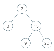
🧩 Approach

To implement the BSTIterator, we can use a stack to simulate the in-order traversal of the binary search tree. The idea is to push all the left children of the current node onto the stack until we reach a leaf node. When we call next(), we pop the top node from the stack, which will be the next smallest element in the BST. After popping a node, we need to consider its right child and push all of its left children onto the stack as well. This way, we maintain the invariant that the top of the stack always contains the next smallest element in the BST.

💡 Solution

from typing import Optional, List

class TreeNode:

    def __init__(self, val=0, left=None, right=None):
        """Initializes a TreeNode with the given value and optional left and right children.

        Args:
            val (int): The value of the node. Default is 0.
            left (Optional[TreeNode]): The left child of the node. Default is None.
            right (Optional[TreeNode]): The right child of the node. Default is None.

        Returns:
            None
        """
        self.val: int = val
        self.left: Optional[TreeNode] = left
        self.right: Optional[TreeNode] = right

class BSTIterator:

    def __init__(self, root: Optional[TreeNode]):
        """Initializes the BSTIterator object with the given root of the binary search tree.

        Args:
            root (Optional[TreeNode]): The root of the binary search tree.

        Returns:
            None
        """
        self.__stack: List[TreeNode] = []
        while root:
            self.__stack.append(root)
            root = root.left

    def next(self) -> int:
        """Moves the pointer to the right, then returns the number at the pointer.

        Args:
            None

        Returns:
            int: The next number in the in-order traversal of the BST.
        """
        res: TreeNode = self.__stack.pop()
        cur: TreeNode = res.right
        while cur:
            self.__stack.append(cur)
            cur = cur.left
        return res.val

    def hasNext(self) -> bool:
        """Returns whether there exists a number in the traversal to the right of the pointer.

        Args:
            None

        Returns:
            bool: True if there exists a next number in the in-order traversal, False otherwise.
        """
        return self.__stack != []

🧮 Complexity Analysis

Time Complexity:
- next: O(1) amortized
- hasNext: O(1)
Space Complexity: O(h) where h is the height of the binary search tree.

208. Implement Trie (Prefix Tree)

LeetCode Link: Implement Trie (Prefix Tree)
Difficulty: Medium
Topic(s): Design, Trie
Company: Microsoft

🧠 Problem Statement

A trie (pronounced as “try”) or prefix tree is a tree data structure used to efficiently store and retrieve keys in a dataset of strings. There are various applications of this data structure, such as autocomplete and spellchecker.

Implement the Trie class:

Trie() Initializes the trie object.

void insert(String word) Inserts the string word into the trie.

boolean search(String word) Returns true if the string word is in the trie (i.e., was inserted before), and false otherwise.

boolean startsWith(String prefix) Returns true if there is a previously inserted string word that has the prefix prefix, and false otherwise.

Example 1:
Input
["Trie", "insert", "search", "search", "startsWith", "insert", "search"]
[[], ["apple"], ["apple"], ["app"], ["app"], ["app"], ["app"]]

Output
[null, null, true, false, true, null, true]

Explanation
Trie trie = new Trie();
trie.insert("apple");
trie.search("apple"); // return True
trie.search("app"); // return False
trie.startsWith("app"); // return True
trie.insert("app");
trie.search("app"); // return True

🧩 Approach

To implement a Trie (Prefix Tree), we can define a TrieNode class that represents each node in the trie. Each TrieNode will contain a dictionary of its children nodes and a boolean flag to indicate whether it represents the end of a word. The Trie class will use the TrieNode to build the trie structure. The insert method will add words to the trie, the search method will check for the existence of a word, and the startsWith method will check for the existence of any word that starts with a given prefix.

💡 Solution

from typing import Dict

class TrieNode:

    def __init__(self):
        """Initializes a TrieNode with an empty dictionary of children and a boolean flag to indicate the end of a word.

        Args:
            None

        Returns:
            None
        """
        self.children: Dict[str, TrieNode] = {}
        self.endOfWord: bool = False

class Trie:

    def __init__(self):
        """Initializes the Trie object.

        Args:
            None

        Returns:
            None
        """
        self.__root = TrieNode()

    def insert(self, word: str) -> None:
        """Inserts the string word into the trie.

        Args:
            word (str): The string to be inserted into the trie.

        Returns:
            None
        """
        cur: TrieNode = self.__root
        for c in word:
            if c not in cur.children:
                cur.children[c] = TrieNode()
            cur = cur.children[c]
        cur.endOfWord = True

    def search(self, word: str) -> bool:
        """Returns true if the string word is in the trie, and false otherwise.

        Args:
            word (str): The string to be searched in the trie.

        Returns:
            bool: True if the string is in the trie, False otherwise.
        """
        cur: TrieNode = self.__root
        for c in word:
            if c not in cur.children:
                return False
            cur = cur.children[c]
        return cur.endOfWord

    def startsWith(self, prefix: str) -> bool:
        """Returns true if there is a previously inserted string word that has the prefix prefix, and false otherwise.

        Args:
            prefix (str): The prefix to be searched in the trie.

        Returns:
            bool: True if there is a string in the trie that starts with the prefix, False otherwise.
        """
        cur: TrieNode = self.__root
        for c in prefix:
            if c not in cur.children:
                return False
            cur = cur.children[c]
        return True

🧮 Complexity Analysis

Time Complexity:
- insert: O(m) where m is the length of the word being inserted.
- search: O(m) where m is the length of the word being searched.
- startsWith: O(m) where m is the length of the prefix being searched.
Space Complexity: O(n * m) where n is the number of words inserted into the trie and m is the average length of the words. In the worst case, if all words are unique and have no common prefixes, the space complexity can be O(n * m). However, if many words share common prefixes, the space complexity can be significantly reduced.

211. Design Add and Search Words Data Structure

LeetCode Link: Design Add and Search Words Data Structure
Difficulty: Medium
Topic(s): Design, Trie, Backtracking
Company: Google

🧠 Problem Statement

Design a data structure that supports adding new words and finding if a string matches any previously added string.

Implement the WordDictionary class:

WordDictionary() Initializes the object.

void addWord(word) Adds word to the data structure, it can be matched later.

bool search(word) Returns true if there is any string in the data structure that matches word or false otherwise. word may contain dots '.' where dots can be matched with any letter.

Example:
Input
["WordDictionary","addWord","addWord","addWord","search","search","search","search"]
[[],["bad"],["dad"],["mad"],["pad"],["bad"],[".ad"],["b.."]]

Output
[null,null,null,null,false,true,true,true]

Explanation
WordDictionary wordDictionary = new WordDictionary();
wordDictionary.addWord("bad");
wordDictionary.addWord("dad");
wordDictionary.addWord("mad");
wordDictionary.search("pad"); // return False
wordDictionary.search("bad"); // return True
wordDictionary.search(".ad"); // return True
wordDictionary.search("b.."); // return True

🧩 Approach

To implement the WordDictionary, we can use a Trie (Prefix Tree) data structure to store the added words. The addWord method will insert words into the trie, while the search method will perform a depth-first search (DFS) to handle the case where the search word may contain dots '.'. When we encounter a dot in the search word, we need to explore all possible child nodes at that position in the trie. If we reach the end of the search word and find a node that marks the end of a valid word, we return true. If we exhaust all possibilities without finding a match, we return false.

💡 Solution

from typing import Dict

class TrieNode:

    def __init__(self):
        """Initializes a TrieNode with an empty dictionary of children and a boolean flag to indicate the end of a word.

        Args:
            None

        Returns:
            None
        """
        self.children: Dict[str, TrieNode] = {}
        self.endOfWord: bool = False

class WordDictionary:

    def __init__(self):
        """Initializes the WordDictionary object.

        Args:
            None

        Returns:
            None
        """
        self.__root = TrieNode()

    def addWord(self, word: str) -> None:
        """Adds word to the data structure, it can be matched later.

        Args:
            word (str): The word to be added to the data structure.

        Returns:
            None
        """
        cur: TrieNode = self.__root
        for c in word:
            if c not in cur.children:
                cur.children[c] = TrieNode()
            cur = cur.children[c]
        cur.endOfWord = True

    def search(self, word: str) -> bool:
        """Returns true if there is any string in the data structure that matches word or false otherwise. word may contain dots '.' where dots can be matched with any letter.

        Args:
            word (str): The word to be searched in the data structure. It may contain dots '.'.

        Returns:
            bool: True if there is a string in the data structure that matches the word, False otherwise.
        """
        def dfs(j, root):
            cur: TrieNode = root
            for i in range(j, len(word)):
                c: str = word[i]
                if c == ".":
                    for child in cur.children.values():
                        if dfs(i + 1, child):
                            return True
                    return False
                else:
                    if c not in cur.children:
                        return False
                    cur = cur.children[c]
            return cur.endOfWord
        return dfs(0, self.__root)

🧮 Complexity Analysis

Time Complexity:
- addWord: O(m) where m is the length of the word being added.
- search: In the worst case, if the search word contains only dots, the time complexity can be O(n * m) where n is the number of words in the data structure and m is the average length of the words. However, if there are fewer dots and more specific characters, the time complexity can be significantly reduced.
Space Complexity: O(n * m) where n is the number of words added to the data structure and m is the average length of the words. In the worst case, if all words are unique and have no common prefixes, the space complexity can be O(n * m). However, if many words share common prefixes, the space complexity can be significantly reduced.

225. Implement Stack using Queues

LeetCode Link: Implement Stack using Queues
Difficulty: Easy
Topic(s): Design, Queue, Stack
Company: Google

🧠 Problem Statement

Implement a last-in-first-out (LIFO) stack using only two queues. The implemented stack should support all the functions of a normal stack (push, top, pop, and empty).

Implement the MyStack class:

void push(int x) Pushes element x to the top of the stack.

int pop() Removes the element on the top of the stack and returns it.

int top() Returns the element on the top of the stack.

boolean empty() Returns true if the stack is empty, false otherwise.

Notes:

You must use only standard operations of a queue, which means that only push to back, peek/pop from front, size and is empty operations are valid.

Depending on your language, the queue may not be supported natively. You may simulate a queue using a list or deque (double-ended queue) as long as you use only a queue’s standard operations.

Example 1:
Input
["MyStack", "push", "push", "top", "pop", "empty"]
[[], [1], [2], [], [], []]

Output
[null, null, null, 2, 2, false]

Explanation
MyStack myStack = new MyStack();
myStack.push(1);
myStack.push(2);
myStack.top(); // return 2
myStack.pop(); // return 2
myStack.empty(); // return False

🧩 Approach

To implement a stack using queues, we can use a single queue to store the elements of the stack. The main idea is to ensure that the most recently added element (the top of the stack) is always at the front of the queue. This way, we can perform pop and top operations in O(1) time. To achieve this, when we pop a new element onto the stack, we can enqueue it to the back of the queue and then rotate the queue by dequeuing all elements before it and enqueuing them back to the end of the queue. This way, the new element will be at the front of the queue, representing the top of the stack.

💡 Solution

from collections import deque

class MyStack:

    def __init__(self):
        """Initializes an empty stack."""
        self.__q: deque[int] = deque()

    def push(self, x: int) -> None:
        """Pushes an element onto the top of the stack.

        Args:
            x (int): The value to be pushed onto the stack.

        Returns:
            None
        """
        self.__q.append(x)

    def pop(self) -> int:
        """Removes and returns the top element of the stack.

        Args:
            None

        Returns:
            int: The element removed from the top of the stack.
        """
        for _ in range(len(self.__q) - 1):
            self.__q.append(self.__q.popleft())
        return self.__q.popleft()


    def top(self) -> int:
        """Returns the top element of the stack without removing it.

        Args:
            None

        Returns:
            int: The element at the top of the stack.
        """
        return self.__q[-1]


    def empty(self) -> bool:
        """Checks whether the stack is empty.

        Args:
            None

        Returns:
            bool: True if the stack is empty, False otherwise.
        """
        return not self.__q

🧮 Complexity Analysis

Time Complexity:
- push: O(1)
- pop: O(n)
- top: O(1)
- empty: O(1)
Space Complexity: O(n)

232. Implement Queue using Stacks

LeetCode Link: Implement Queue using Stacks
Difficulty: Easy
Topic(s): Design, Queue, Stack
Company: Microsoft

🧠 Problem Statement

Implement a first in first out (FIFO) queue using only two stacks. The implemented queue should support all the functions of a normal queue (push, peek, pop, and empty).

Implement the MyQueue class:

void push(int x) Pushes element x to the back of the queue.

int pop() Removes the element from the front of the queue and returns it.

int peek() Returns the element at the front of the queue.

boolean empty() Returns true if the queue is empty, false otherwise.

Notes:

You must use only standard operations of a stack, which means only push to top, peek/pop from top, size, and is empty operations are valid. Depending on your language, the stack may not be supported natively. You may simulate a stack using a list or deque (double-ended queue) as long as you use only a stack’s standard operations.

Example 1:
Input
["MyQueue", "push", "push", "peek", "pop", "empty"]
[[], [1], [2], [], [], []]

Output
[null, null, null, 1, 1, false]

Explanation
MyQueue myQueue = new MyQueue();
myQueue.push(1); // queue is: [1]
myQueue.push(2); // queue is: [1, 2] (leftmost is front of the queue)
myQueue.peek(); // return 1
myQueue.pop(); // return 1, queue is [2]
myQueue.empty(); // return false

🧩 Approach

To implement a queue using stacks, we can use two stacks to manage the elements of the queue. The main idea is to use one stack (s1) for enqueueing elements and another stack (s2) for dequeueing elements. When we need to dequeue an element, if s2 is empty, we can pop all elements from s1 and push them onto s2, which will reverse the order of the elements and allow us to access the front of the queue. This way, we can perform push, pop, and peek operations efficiently.

💡 Solution

from typing import List

class MyQueue:

    def __init__(self):
        """Initializes an empty queue using two stacks."""
        self.__s1: List[int] = []
        self.__s2: List[int] = []

    def push(self, x: int) -> None:
        """Pushes an element to the back of the queue.

        Args:
            x (int): The value to be pushed onto the queue.

        Returns:
            None
        """
        self.__s1.append(x)

    def pop(self) -> int:
        """Removes and returns the front element of the queue.

        Args:
            None

        Returns:
            int: The element removed from the front of the queue.
        """
        if not self.__s2:
            while self.__s1:
                self.__s2.append(self.__s1.pop())
        return self.__s2.pop()

    def peek(self) -> int:
        """Returns the front element of the queue without removing it.

        Args:
            None

        Returns:
            int: The element at the front of the queue.
        """
        if not self.__s2:
            while self.__s1:
                self.__s2.append(self.__s1.pop())
        return self.__s2[-1]

    def empty(self) -> bool:
        """Checks whether the queue is empty.

        Args:
            None

        Returns:
            bool: True if the queue is empty, False otherwise.
        """
        return max(len(self.__s1), len(self.__s2)) == 0

🧮 Complexity Analysis

Time Complexity:
- push: O(1)
- pop: O(1) amortized
- peek: O(1) amortized
- empty: O(1)
Space Complexity: O(n)

284. Peeking Iterator

LeetCode Link: Peeking Iterator
Difficulty: Medium
Topic(s): Design, Iterator
Company: Google

🧠 Problem Statement

Design an iterator that supports the peek operation on an existing iterator in addition to the hasNext and the next operations.

Implement the PeekingIterator class:

PeekingIterator(Iterator<int> nums) Initializes the object with the given integer iterator iterator.

int next() Returns the next element in the array and moves the pointer to the next element.

boolean hasNext() Returns true if there are still elements in the array.

int peek() Returns the next element in the array without moving the pointer.

Note: Each language may have a different implementation of the constructor and Iterator, but they all support the int next() and boolean hasNext() functions.

Example 1:
Input
["PeekingIterator", "next", "peek", "next", "next", "hasNext"]
[[[1, 2, 3]], [], [], [], [], []]
Output
[null, 1, 2, 2, 3, false]

Explanation
PeekingIterator peekingIterator = new PeekingIterator([1, 2, 3]); // [1,2,3]
peekingIterator.next(); // return 1, the pointer moves to the next element [1,2,3].
peekingIterator.peek(); // return 2, the pointer does not move [1,2,3].
peekingIterator.next(); // return 2, the pointer moves to the next element [1,2,3]
peekingIterator.next(); // return 3, the pointer moves to the next element [1,2,3]
peekingIterator.hasNext(); // return False

🧩 Approach

To implement the PeekingIterator, we can maintain a cache to store the next element of the iterator. This way, we can return the next element in constant time when peek() is called without advancing the iterator. When next() is called, we can return the cached value and then update the cache with the next element from the iterator. The hasNext() method can simply check if there is a cached value available.

💡 Solution

# Below is the interface for Iterator, which is already defined for you.
#
# class Iterator:
#     def __init__(self, nums):
#         """Initializes an iterator object to the beginning of a list.
#
#         Args:
#             nums (List[int]): The list of integers to iterate over.
#
#         Returns:
#             None
#         """
#
#     def hasNext(self):
#         """Returns true if the iteration has more elements.
#
#         Args:
#             None
#
#         Returns:
#             bool: True if there are more elements to iterate over, False otherwise.
#         """
#
#     def next(self):
#         """Returns the next element in the iteration.
#
#         Args:
#             None
#         Returns:
#             int: The next element in the iteration.
#         """

class PeekingIterator:
    def __init__(self, iterator):
        """Initializes the PeekingIterator with the given iterator.

        Args:
            iterator (Iterator): The input iterator to be wrapped by the PeekingIterator.

        Returns:
            None
        """
        self.__iterator: Iterator = iterator
        self.__cache: int = None
        self.__peekCache()

    def __peekCache(self) -> None:
        """Updates the cache with the next element from the iterator if it exists, otherwise sets it to None.

        Args:
            None

        Returns:
            None
        """
        if self.__iterator.hasNext():
            self.__cache = self.__iterator.next()
        else:
            self.__cache = None

    def peek(self):
        """Returns the next element in the array without moving the pointer.

        Args:
            None

        Returns:
            int: The next element in the array.
        """
        return self.__cache

    def next(self) -> int:
        """Returns the next element in the array and moves the pointer to the next element.

        Args:
            None

        Returns:
            int: The next element in the array.
        """
        peek: int = self.__cache
        self.__peekCache()
        return peek

    def hasNext(self) -> bool:
        """Returns true if there are still elements in the array.

        Args:
            None

        Returns:
            bool: True if there are still elements in the array, False otherwise.
        """
        return self.__cache is not None

🧮 Complexity Analysis

Time Complexity:
- peek: O(1)
- next: O(1)
- hasNext: O(1)
Space Complexity: O(1)

303. Range Sum Query - Immutable

LeetCode Link: Range Sum Query - Immutable
Difficulty: Easy
Topic(s): Design, Array, Prefix Sum
Company: Amazon

🧠 Problem Statement

Given an integer array nums, handle multiple queries of the following type:

Calculate the sum of the elements of nums between indices left and right inclusive where left <= right.

Implement the NumArray class:

NumArray(int[] nums) Initializes the object with the integer array nums.

int sumRange(int left, int right) Returns the sum of the elements of nums between indices left and right inclusive (i.e. nums[left] + nums[left + 1] + ... + nums[right]).

Example 1:
Input
["NumArray", "sumRange", "sumRange", "sumRange"]
[[[-2, 0, 3, -5, 2, -1]], [0, 2], [2, 5], [0, 5]]

Output
[null, 1, -1, -3]

Explanation
NumArray numArray = new NumArray([-2, 0, 3, -5, 2, -1]);
numArray.sumRange(0, 2); // return (-2) + 0 + 3 = 1
numArray.sumRange(2, 5); // return 3 + (-5) + 2 + (-1) = -1
numArray.sumRange(0, 5); // return (-2) + 0 + 3 + (-5) + 2 + (-1) = -3

🧩 Approach

To efficiently calculate the sum of elements in a given range, we can use a prefix sum array. The prefix sum array allows us to compute the sum of any subarray in constant time after an initial preprocessing step. The idea is to create a prefix sum array where each element at index i contains the sum of all elements from the start of the original array up to index i. Then, to calculate the sum of elements between indices left and right, we can simply subtract the prefix sum at left - 1 from the prefix sum at right.

💡 Solution

from typing import List

class NumArray:

    def __init__(self, nums: List[int]):
        """Initializes the NumArray object with the given integer array.

        Args:
            nums (List[int]): The input integer array.

        Returns:
            None
        """
        self.__prefix: List[int] = []
        cur: int = 0
        for n in nums:
            cur += n
            self.__prefix.append(cur)

    def sumRange(self, left: int, right: int) -> int:
        """Returns the sum of the elements of nums between indices left and right inclusive.

        Args:
            left (int): The starting index of the range.
            right (int): The ending index of the range.

        Returns:
            int: The sum of the elements in the specified range.
        """
        rightSum: int = self.__prefix[right]
        leftSum: int = self.__prefix[left - 1] if left > 0 else 0
        return rightSum - leftSum

🧮 Complexity Analysis

Time Complexity:
- __init__: O(n) for preprocessing the prefix sum array.
- sumRange: O(1) for each query after preprocessing.
Space Complexity: O(n)

304. Range Sum Query 2D - Immutable

LeetCode Link: Range Sum Query 2D - Immutable
Difficulty: Medium
Topic(s): Design, Array, Prefix Sum
Company: Amazon

🧠 Problem Statement

Given a 2D matrix matrix, handle multiple queries of the following type:

Calculate the sum of the elements of matrix inside the rectangle defined by its upper left corner (row1, col1) and lower right corner (row2, col2).

Implement the NumMatrix class:

NumMatrix(int[][] matrix) Initializes the object with the integer matrix matrix.

int sumRegion(int row1, int col1, int row2, int col2) Returns the sum of the elements of matrix inside the rectangle defined by its upper left corner (row1, col1) and lower right corner (row2, col2).

You must design an algorithm where sumRegion works on O(1) time complexity.

Example 1:
Input
["NumMatrix", "sumRegion", "sumRegion", "sumRegion"]
[[[[3, 0, 1, 4, 2], [5, 6, 3, 2, 1], [1, 2, 0, 1, 5], [4, 1, 0, 1, 7], [1, 0, 3, 0, 5]]], [2, 1, 4, 3], [1, 1, 2, 2], [1, 2, 2, 4]]

Output
[null, 8, 11, 12]

Explanation
NumMatrix numMatrix = new NumMatrix([[3, 0, 1, 4, 2], [5, 6, 3, 2, 1], [1, 2, 0, 1, 5], [4, 1, 0, 1, 7], [1, 0, 3, 0, 5]]);
numMatrix.sumRegion(2, 1, 4, 3); // return 8 (i.e sum of the red rectangle)
numMatrix.sumRegion(1, 1, 2, 2); // return 11 (i.e sum of the green rectangle)
numMatrix.sumRegion(1, 2, 2, 4); // return 12 (i.e sum of the blue rectangle)

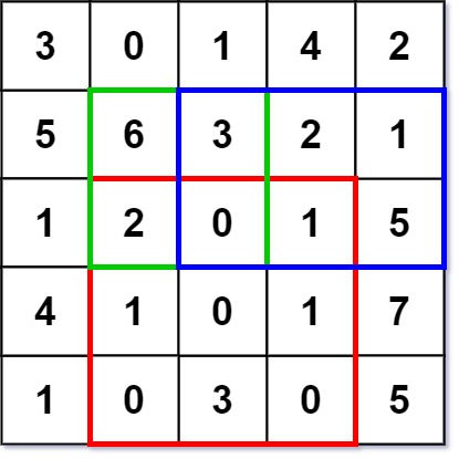
🧩 Approach

To efficiently calculate the sum of elements in a given rectangular region of a 2D matrix, we can use a 2D prefix sum matrix. The prefix sum matrix allows us to compute the sum of any submatrix in constant time after an initial preprocessing step. The idea is to create a prefix sum matrix where each element at index (i, j) contains the sum of all elements from the top-left corner of the original matrix up to index (i, j). Then, to calculate the sum of elements in the rectangle defined by (row1, col1) and (row2, col2), we can use the inclusion-exclusion principle to combine the relevant prefix sums.

💡 Solution

from typing import List

class NumMatrix:

    def __init__(self, matrix: List[List[int]]):
        """Initializes the NumMatrix object with the given 2D integer matrix.

        Args:
            matrix (List[List[int]]): The input 2D integer matrix.

        Returns:
            None
        """
        R, C = len(matrix), len(matrix[0])
        self.__sumMat: List[List[int]] = [[0] * (C + 1) for _ in range(R + 1)]

        for r in range(R):
            prefix: int = 0
            for c in range(C):
                prefix += matrix[r][c]
                above: int = self.__sumMat[r][c + 1]
                self.__sumMat[r + 1][c + 1] = prefix + above

    def sumRegion(self, row1: int, col1: int, row2: int, col2: int) -> int:
        """Returns the sum of the elements of matrix inside the rectangle defined by its upper left corner (row1, col1) and lower right corner (row2, col2).

        Args:
            row1 (int): The row index of the upper left corner of the rectangle.
            col1 (int): The column index of the upper left corner of the rectangle.
            row2 (int): The row index of the lower right corner of the rectangle.
            col2 (int): The column index of the lower right corner of the rectangle.

        Returns:
            int: The sum of the elements in the specified rectangle.
        """
        row1, col1, row2, col2 = row1 + 1, col1 + 1, row2 + 1, col2 + 1

        bottomRight: int = self.__sumMat[row2][col2]
        above: int = self.__sumMat[row1 - 1][col2]
        left: int = self.__sumMat[row2][col1 - 1]
        topLeft: int = self.__sumMat[row1 - 1][col1 - 1]

        return bottomRight - above - left + topLeft

🧮 Complexity Analysis

Time Complexity:
- __init__: O(R * C) for preprocessing the prefix sum matrix.
- sumRegion: O(1) for each query after preprocessing.
Space Complexity: O(R * C) for storing the prefix sum matrix.

307. Range Sum Query - Mutable

LeetCode Link: Range Sum Query - Mutable
Difficulty: Medium
Topic(s): Design, Array, Segment Tree, Binary Indexed Tree
Company: Amazon

🧠 Problem Statement

Given an integer array nums, handle multiple queries of the following types:

Update the value of an element in nums.

Calculate the sum of the elements of nums between indices left and right inclusive where left <= right.

Implement the NumArray class:

NumArray(int[] nums) Initializes the object with the integer array nums.

void update(int index, int val) Updates the value of nums[index] to be val.

int sumRange(int left, int right) Returns the sum of the elements of nums between indices left and right inclusive (i.e. nums[left] + nums[left + 1] + ... + nums[right]).

Example 1:
Input
["NumArray", "sumRange", "update", "sumRange"]
[[[1, 3, 5]], [0, 2], [1, 2], [0, 2]]

Output
[null, 9, null, 8]

Explanation
NumArray numArray = new NumArray([1, 3, 5]);
numArray.sumRange(0, 2); // return 1 + 3 + 5 = 9
numArray.update(1, 2); // nums = [1, 2, 5]
numArray.sumRange(0, 2); // return 1 + 2 + 5 = 8

🧩 Approach

To efficiently handle updates and range sum queries on an array, we can use a Segment Tree data structure. A Segment Tree allows us to perform both update and query operations in logarithmic time. The idea is to build a binary tree where each node represents a segment of the array and stores the sum of that segment. When we need to update an element, we can update the corresponding leaf node and then propagate the changes up the tree. When we need to calculate the sum of a range, we can traverse the tree and combine the sums of the relevant segments.

💡 Solution

from typing import List

class Node:
    def __init__(self, start, end):
        """Initializes a Node in the Segment Tree with the given start and end indices.

        Args:
            start (int): The starting index of the segment represented by this node.
            end (int): The ending index of the segment represented by this node.

        Returns:
            None
        """
        self.start: int = start
        self.end: int = end
        self.total: int = 0
        self.left: Node = None
        self.right: Node = None


class NumArray:

    def __init__(self, nums: List[int]):
        """Initializes the NumArray object with the given integer array.

        Args:
            nums (List[int]): The input integer array.

        Returns:
            None
        """
        def createTree(nums: List[int], l: int, r: int) -> Node:
            """Recursively builds a segment tree from the input array nums between indices l and r.

            Args:
                nums (List[int]): The input array of integers.
                l (int): The left index of the current segment.
                r (int): The right index of the current segment.

            Returns:
                Node: The root node of the segment tree for the current segment.
            """
            if l > r:
                return None

            if l == r:
                n: Node = Node(l, r)
                n.total = nums[l]
                return n

            mid: int = (l + r) // 2
            root: Node = Node(l, r)

            root.left = createTree(nums, l, mid)
            root.right = createTree(nums, mid + 1, r)

            root.total = root.left.total + root.right.total

            return root

        self.root: Node = createTree(nums, 0, len(nums) - 1)

    def update(self, index: int, val: int) -> None:
        """Updates the value at the specified index in the array and updates the segment tree accordingly.

        Args:
            index (int): The index of the element to be updated.
            val (int): The new value to be set at the specified index.

        Returns:
            None
        """
        def updateVal(root: Node, i: int, val: int) -> int:
            """Recursively updates the value at index i in the segment tree rooted at root and updates the total values of the affected nodes.

            Args:
                root (Node): The current node in the segment tree.
                i (int): The index of the element to be updated.
                val (int): The new value to be set at the specified index.

            Returns:
                int: The updated total value of the current node after the update.
            """
            if root.left == root.right:
                root.total = val
                return val

            mid: int = (root.start + root.end) // 2

            if i <= mid:
                updateVal(root.left, i, val)
            else:
                updateVal(root.right, i, val)

            root.total = root.left.total + root.right.total

            return root.total

        updateVal(self.root, index, val)

    def sumRange(self, left: int, right: int) -> int:
        """Returns the sum of the elements of the array between indices left and right inclusive.

        Args:
            left (int): The starting index of the range.
            right (int): The ending index of the range.

        Returns:
            int: The sum of the elements in the specified range.
        """
        def rangeSum(root: Node, i: int, j: int) -> int:
            """Recursively calculates the sum of the elements in the range [i, j] in the segment tree rooted at root.

            Args:
                root (Node): The current node in the segment tree.
                i (int): The starting index of the range.
                j (int): The ending index of the range.

            Returns:
                int: The sum of the elements in the specified range.
            """
            if root.start == i and root.end == j:
                return root.total

            mid: int = (root.start + root.end) // 2

            if j <= mid:
                return rangeSum(root.left, i, j)

            elif i >= mid + 1:
                return rangeSum(root.right, i, j)

            else:
                return rangeSum(root.left, i, mid) + rangeSum(root.right, mid + 1, j)

        return rangeSum(self.root, left, right)

🧮 Complexity Analysis

Time Complexity:
- __init__: O(n) for building the segment tree.
- update: O(log n) for updating an element in the segment tree.
- sumRange: O(log n) for querying the sum of a range in the segment tree.
Space Complexity: O(n) for storing the segment tree.

341. Flatten Nested List Iterator

LeetCode Link: Flatten Nested List Iterator
Difficulty: Medium
Topic(s): Design, Stack, Iterator
Company: Google

🧠 Problem Statement

You are given a nested list of integers nestedList. Each element is either an integer or a list whose elements may also be integers or other lists. Implement an iterator to flatten it.

Implement the NestedIterator class:

NestedIterator(List<NestedInteger> nestedList): Initializes the iterator with the nested list nestedList.

int next(): Returns the next integer in the nested list.

boolean hasNext(): Returns true if there are still some integers in the nested list and false otherwise.

Your code will be tested with the following pseudocode:
initialize iterator with nestedList
res = []
while iterator.hasNext()
append iterator.next() to the end of res
return res
If res matches the expected flattened list, then your code will be judged as correct.

Example 1:
Input: nestedList = [[1,1],2,[1,1]]

Output: [1,1,2,1,1]

Explanation: By calling next repeatedly until hasNext returns false, the order of elements returned by next should be: [1,1,2,1,1].
Example 2:
Input: nestedList = [1,[4,[6]]]

Output: [1,4,6]

Explanation: By calling next repeatedly until hasNext returns false, the order of elements returned by next should be: [1,4,6].

🧩 Approach

To implement the NestedIterator, we can use a depth-first search (DFS) approach to flatten the nested list of integers. We can maintain a stack to store the integers in the order they should be returned. During the initialization, we can perform a DFS on the input nested list and push all the integers onto the stack. After the DFS is complete, we can reverse the stack to ensure that the integers are in the correct order for iteration. The next() method will simply pop an integer from the stack, and the hasNext() method will check if there are any integers left in the stack.

💡 Solution

from typing import List

# """
# This is the interface that allows for creating nested lists.
# You should not implement it, or speculate about its implementation
# """
#class NestedInteger:
#    def isInteger(self) -> bool:
#        """
#        @return True if this NestedInteger holds a single integer, rather than a nested list.
#        """
#
#    def getInteger(self) -> int:
#        """
#        @return the single integer that this NestedInteger holds, if it holds a single integer
#        Return None if this NestedInteger holds a nested list
#        """
#
#    def getList(self) -> [NestedInteger]:
#        """
#        @return the nested list that this NestedInteger holds, if it holds a nested list
#        Return None if this NestedInteger holds a single integer
#        """

class NestedIterator:
    def __init__(self, nestedList: [NestedInteger]):
        """Initializes the NestedIterator with the given nested list.

        Args:
            nestedList (List[NestedInteger]): The input nested list of integers.

        Returns:
            None
        """
        self.stack: List[int] = []
        self.dfs(nestedList)
        self.stack.reverse()


    def next(self) -> int:
        """Returns the next integer in the nested list.

        Args:
            None

        Returns:
            int: The next integer in the nested list.
        """
        return self.stack.pop()


    def hasNext(self) -> bool:
        """Returns true if there are still some integers in the nested list and false otherwise.

        Args:
            None

        Returns:
            bool: True if there are still some integers in the nested list, False otherwise.
        """
        return len(self.stack) > 0

    def dfs(self, nested: NestedInteger):
        """Performs a depth-first search on the nested list to flatten it and store the integers in the stack.

        Args:
            nested (NestedInteger): The current nested list or integer to be processed.

        Returns:
            None
        """
        for n in nested:
            if n.isInteger():
                self.stack.append(n.getInteger())
            else:
                self.dfs(n.getList())

🧮 Complexity Analysis

Time Complexity:
- __init__: O(n) for flattening the nested list, where n is the total number of integers in the nested list.
- next: O(1) for returning the next integer.
- hasNext: O(1) for checking if there are more integers to return.
Space Complexity: O(n) for storing the flattened integers in the stack.

355. Design Twitter

LeetCode Link: Design Twitter
Difficulty: Medium
Topic(s): Design, Hash Table, Heap, Priority Queue

🧠 Problem Statement

Design a simplified version of Twitter where users can post tweets, follow/unfollow another user, and is able to see the 10 most recent tweets in the user’s news feed.

Implement the Twitter class:

Twitter() Initializes your twitter object.

void postTweet(int userId, int tweetId) Composes a new tweet with ID tweetId by the user with ID userId. Each call to this function will be made with a unique tweetId.

List<Integer> getNewsFeed(int userId) Retrieves the 10 most recent tweet IDs in the user’s news feed. Each item in the news feed must be posted by users who the user followed or by the user themself. Tweets must be ordered from most recent to least recent.

void follow(int followerId, int followeeId) The user with ID followerId started following the user with ID followeeId.

void unfollow(int followerId, int followeeId) The user with ID followerId started unfollowing the user with ID followeeId.

Example 1:
Input
["Twitter", "postTweet", "getNewsFeed", "follow", "postTweet", "getNewsFeed", "unfollow", "getNewsFeed"]
[[], [1, 5], [1], [1, 2], [2, 6], [1], [1, 2], [1]]

Output
[null, null, [5], null, null, [6, 5], null, [5]]

Explanation
Twitter twitter = new Twitter();
twitter.postTweet(1, 5); // User 1 posts a new tweet (id = 5).
twitter.getNewsFeed(1); // User 1's news feed should return a list with 1 tweet id -> [5]. return [5]
twitter.follow(1, 2); // User 1 follows user 2.
twitter.postTweet(2, 6); // User 2 posts a new tweet (id = 6).
twitter.getNewsFeed(1); // User 1's news feed should return a list with 2 tweet ids -> [6, 5]. Tweet id 6 should precede tweet id 5 because it is posted after tweet id 5.
twitter.unfollow(1, 2); // User 1 unfollows user 2.
twitter.getNewsFeed(1); // User 1's news feed should return a list with 1 tweet id -> [5], since user 1 is no longer following user 2.

🧩 Approach

To design the Twitter class, we can use a combination of hash maps and a min-heap (priority queue) to efficiently manage tweets and follow relationships. We will maintain a mapping of user IDs to their tweets, as well as a mapping of user IDs to the set of users they follow. When retrieving the news feed for a user, we can use a min-heap to merge the most recent tweets from the user and their followees, ensuring that we return the 10 most recent tweets in the correct order.

💡 Solution

import heapq
from collections import defaultdict
from typing import Dict, List, Set


class Twitter:
    """A simplified Twitter-like social media system.

    Supports posting tweets, following/unfollowing users,
    and retrieving a user's news feed of the 10 most recent tweets
    from themselves and the users they follow.

    Attributes:
        count (int): A counter used to order tweets by recency (decrements on each post).
        tweetMap (Dict[int, List[List[int]]]): Maps each userId to a list of [count, tweetId] pairs.
        followMap (Dict[int, Set[int]]): Maps each userId to the set of followeeIds they follow.
    """

    def __init__(self) -> None:
        """Initializes the Twitter system with empty tweet and follow maps."""
        self.count: int = 0
        self.tweetMap: Dict[int, List[List[int]]] = defaultdict(list)
        self.followMap: Dict[int, Set[int]] = defaultdict(set)

    def postTweet(self, userId: int, tweetId: int) -> None:
        """Posts a new tweet for the given user.

        Args:
            userId (int): The ID of the user posting the tweet.
            tweetId (int): The ID of the tweet being posted.
        """
        self.tweetMap[userId].append([self.count, tweetId])
        self.count -= 1

    def getNewsFeed(self, userId: int) -> List[int]:
        """Retrieves the 10 most recent tweet IDs from the user's news feed.

        The feed includes tweets from the user themselves and all users they follow,
        sorted in descending order of recency (most recent first).

        Args:
            userId (int): The ID of the user requesting the news feed.

        Returns:
            List[int]: A list of up to 10 tweet IDs, ordered from most recent to least recent.
        """
        res: List[int] = []
        # Min-heap entries are: [count, tweetId, followeeId, index]
        # 'count' is negative so lower values = more recent tweets (min-heap acts as max-heap)
        minHeap: List[List[int]] = []

        # Ensure the user sees their own tweets by adding themselves to their follow set
        self.followMap[userId].add(userId)

        # Seed the heap with the most recent tweet from each followee
        for followeeId in self.followMap[userId]:
            if followeeId in self.tweetMap:
                # Start from the last (most recent) tweet in the followee's list
                index: int = len(self.tweetMap[followeeId]) - 1
                count, tweetId = self.tweetMap[followeeId][index]
                # Push [count, tweetId, followeeId, next_index] so we can walk backwards later
                minHeap.append([count, tweetId, followeeId, index - 1])

        # Transform the list into a valid heap in O(n)
        heapq.heapify(minHeap)

        # Pop the most recent tweet globally, then push the previous tweet from the same user
        while minHeap and len(res) < 10:
            count, tweetId, followeeId, index = heapq.heappop(minHeap)

            # Add the popped tweet to results
            res.append(tweetId)

            # If this followee has older tweets remaining, push the next one onto the heap
            if index >= 0:
                count, tweetId = self.tweetMap[followeeId][index]
                heapq.heappush(minHeap, [count, tweetId, followeeId, index - 1])

        return res

    def follow(self, followerId: int, followeeId: int) -> None:
        """Makes a user follow another user.

        Args:
            followerId (int): The ID of the user who wants to follow.
            followeeId (int): The ID of the user to be followed.
        """
        self.followMap[followerId].add(followeeId)

    def unfollow(self, followerId: int, followeeId: int) -> None:
        """Makes a user unfollow another user.

        Args:
            followerId (int): The ID of the user who wants to unfollow.
            followeeId (int): The ID of the user to be unfollowed.
        """
        if followeeId in self.followMap[followerId]:
            self.followMap[followerId].remove(followeeId)

🧮 Complexity Analysis

Time Complexity:
- postTweet: O(1) for appending a new tweet.
- getNewsFeed: O(k log n) where k is the number of followees (including self) and n is the average number of tweets per followee, due to heap operations.
- follow: O(1) for adding a followee.
- unfollow: O(1) for removing a followee.
Space Complexity: O(u + t) where u is the number of users and t is the total number of tweets, due to storing follow relationships and tweets.

703. Kth Largest Element in a Stream

LeetCode Link: Kth Largest Element in a Stream
Difficulty: Easy
Topic(s): Design, Heap, Priority Queue
Company: Amazon

🧠 Problem Statement

You are part of a university admissions office and need to keep track of the kth highest test score from applicants in real-time. This helps to determine cut-off marks for interviews and admissions dynamically as new applicants submit their scores.

You are tasked to implement a class which, for a given integer k, maintains a stream of test scores and continuously returns the kth highest test score after a new score has been submitted. More specifically, we are looking for the kth highest score in the sorted list of all scores.

Implement the KthLargest class:

KthLargest(int k, int[] nums) Initializes the object with the integer k and the stream of test scores nums.

int add(int val) Adds a new test score val to the stream and returns the element representing the kth largest element in the pool of test scores so far.

Example 1:
Input:
["KthLargest", "add", "add", "add", "add", "add"]
[[3, [4, 5, 8, 2]], [3], [5], [10], [9], [4]]

Output: [null, 4, 5, 5, 8, 8]

Explanation:

KthLargest kthLargest = new KthLargest(3, [4, 5, 8, 2]);
kthLargest.add(3); // return 4
kthLargest.add(5); // return 5
kthLargest.add(10); // return 5
kthLargest.add(9); // return 8
kthLargest.add(4); // return 8
Example 2:
Input:
["KthLargest", "add", "add", "add", "add"]
[[4, [7, 7, 7, 7, 8, 3]], [2], [10], [9], [9]]

Output: [null, 7, 7, 7, 8]

Explanation:

KthLargest kthLargest = new KthLargest(4, [7, 7, 7, 7, 8, 3]);
kthLargest.add(2); // return 7
kthLargest.add(10); // return 7
kthLargest.add(9); // return 7
kthLargest.add(9); // return 8

🧩 Approach

To maintain the kth largest element in a stream of test scores, we can use a min-heap (priority queue) to store the top k largest elements. The min-heap allows us to efficiently keep track of the smallest element among the top k elements, which will be the kth largest element in the stream. When a new score is added, we can compare it with the smallest element in the heap. If the new score is larger than the smallest element, we can remove the smallest element and add the new score to the heap. This way, we ensure that the heap always contains the k largest elements from the stream.

💡 Solution

from typing import List

import heapq

class KthLargest:

    def __init__(self, k: int, nums: List[int]):
        """Initializes the KthLargest object with the given integer k and the stream of test scores nums.

        Args:
            k (int): The integer k representing the rank of the largest element to maintain.
            nums (List[int]): The initial stream of test scores.

        Returns:
            None
        """
        self.__minHeap: List[int] = nums
        self.__k: int = k
        heapq.heapify(self.__minHeap)
        while len(self.__minHeap) > k:
            heapq.heappop(self.__minHeap)

    def add(self, val: int) -> int:
        """Adds a new test score val to the stream and returns the element representing the kth largest element in the pool of test scores so far.

        Args:
            val (int): The new test score to be added to the stream.

        Returns:
            int: The kth largest element in the stream after adding the new score.
        """
        heapq.heappush(self.__minHeap, val)
        if len(self.__minHeap) > self.__k:
            heapq.heappop(self.__minHeap)
        return self.__minHeap[0]

🧮 Complexity Analysis

Time Complexity:
- __init__: O(n log k) for building the heap and maintaining the top k elements.
- add: O(log k) for adding a new score and maintaining the heap.
Space Complexity: O(k) for storing the top k elements in the heap.

705. Design HashSet

LeetCode Link: Design HashSet
Difficulty: Easy
Topic(s): Design, Hash Table
Company: Meta

🧠 Problem Statement

Design a HashSet without using any built-in hash table libraries.

Implement MyHashSet class:

void add(key) Inserts the value key into the HashSet.

bool contains(key) Returns whether the value key exists in the HashSet or not.

void remove(key) Removes the value key in the HashSet. If key does not exist in the HashSet, do nothing.

Example 1:
Input
["MyHashSet", "add", "add", "contains", "contains", "add", "contains", "remove", "contains"]
[[], [1], [2], [1], [3], [2], [2], [2], [2]]

Output
[null, null, null, true, false, null, true, null, false]

Explanation
MyHashSet myHashSet = new MyHashSet();
myHashSet.add(1); // set = [1]
myHashSet.add(2); // set = [1, 2]
myHashSet.contains(1); // return True
myHashSet.contains(3); // return False, (not found)
myHashSet.add(2); // set = [1, 2]
myHashSet.contains(2); // return True
myHashSet.remove(2); // set = [1]
myHashSet.contains(2); // return False, (already removed)

🧩 Approach

To design a HashSet, we can use an array of linked lists (chaining) to handle collisions. We can define a ListNode class to represent each node in the linked list, which will store the key and a reference to the next node. The MyHashSet class will contain an array of ListNode objects, where each index corresponds to a hash value derived from the key. When adding a key, we will compute its hash value and insert it into the corresponding linked list. For checking if a key exists or for removing a key, we will traverse the linked list at the computed hash index to find the key.

💡 Solution

from typing import Optional, List

class ListNode:

    def __init__(self, key: int):
        """Initializes a ListNode with the given key.

        Args:
            key (int): The value to be stored in the ListNode.

        Returns:
            None
        """
        self.key: int = key
        self.next: Optional[ListNode] = None

class MyHashSet:

    def __init__(self):
        """Initializes an empty HashSet."""
        self.__set: List[ListNode] = [ListNode(0) for _ in range(10**4)]

    def add(self, key: int) -> None:
        """Inserts the value key into the HashSet.

        Args:
            key (int): The value to be added to the HashSet.

        Returns:
            None
        """
        cur: ListNode = self.__set[key % len(self.__set)]
        while cur.next:
            if cur.next.key == key:
                return None
            cur = cur.next
        cur.next = ListNode(key)

    def remove(self, key: int) -> None:
        """Removes the value key in the HashSet. If key does not exist in the HashSet, do nothing.

        Args:
            key (int): The value to be removed from the HashSet.

        Returns:
            None
        """
        cur: ListNode = self.__set[key % len(self.__set)]
        while cur.next:
            if cur.next.key == key:
                cur.next = cur.next.next
                return None
            cur = cur.next

    def contains(self, key: int) -> bool:
        """Returns whether the value key exists in the HashSet or not.

        Args:
            key (int): The value to check for existence in the HashSet.

        Returns:
            bool: True if the value exists in the HashSet, False otherwise.
        """
        cur: ListNode = self.__set[key % len(self.__set)]
        while cur.next:
            if cur.next.key == key:
                return True
            cur = cur.next
        return False

🧮 Complexity Analysis

Time Complexity:
- add: O(1) on average, but O(n) in the worst case due to collision handling with chaining.
- remove: O(1) on average, but O(n) in the worst case due to collision handling with chaining.
- contains: O(1) on average, but O(n) in the worst case due to collision handling with chaining.
Space Complexity: O(n)

706. Design HashMap

LeetCode Link: Design HashMap
Difficulty: Easy
Topic(s): Design, Hash Table
Company: Google

🧠 Problem Statement

Design a HashMap without using any built-in hash table libraries.

Implement the MyHashMap class:

MyHashMap() initializes the object with an empty map.

void put(int key, int value) inserts a (key, value) pair into the HashMap. If the key already exists in the map, update the corresponding value.

int get(int key) returns the value to which the specified key is mapped, or -1 if this map contains no mapping for the key.

void remove(key) removes the key and its corresponding value if the map contains the mapping for the key.

Example 1:
Input
["MyHashMap", "put", "put", "get", "get", "put", "get", "remove", "get"]
[[], [1, 1], [2, 2], [1], [3], [2, 1], [2], [2], [2]]

Output
[null, null, null, 1, -1, null, 1, null, -1]

Explanation
MyHashMap myHashMap = new MyHashMap();
myHashMap.put(1, 1); // The map is now [[1,1]]
myHashMap.put(2, 2); // The map is now [[1,1], [2,2]]
myHashMap.get(1); // return 1, The map is now [[1,1], [2,2]]
myHashMap.get(3); // return -1 (i.e., not found), The map is now [[1,1], [2,2]]
myHashMap.put(2, 1); // The map is now [[1,1], [2,1]] (i.e., update the existing value)
myHashMap.get(2); // return 1, The map is now [[1,1], [2,1]]
myHashMap.remove(2); // remove the mapping for 2, The map is now [[1,1]]
myHashMap.get(2); // return -1 (i.e., not found), The map is now [[1,1]]

🧩 Approach

To design a HashMap, we can use an array of linked lists (chaining) to handle collisions, similar to the design of a HashSet. We can define a ListNode class to represent each node in the linked list, which will store the key, value, and a reference to the next node. The MyHashMap class will contain an array of ListNode objects, where each index corresponds to a hash value derived from the key. When adding a key-value pair, we will compute its hash value and insert it into the corresponding linked list. For checking if a key exists or for removing a key, we will traverse the linked list at the computed hash index to find the key and perform the necessary operations.

💡 Solution

from typing import Optional, List

class ListNode:

    def __init__(self, key: int, value: int):
        self.key: int = key
        self.value: int = value
        self.next: Optional[ListNode] = None

class MyHashMap:

    def __init__(self):
        self.__map: List[ListNode] = [ListNode(0, 0) for _ in range(10**4)]

    def put(self, key: int, value: int) -> None:
        cur: ListNode = self.__map[key % len(self.__map)]
        while cur.next:
            if cur.next.key == key:
                cur.next.value = value
                return None
            cur = cur.next
        cur.next = ListNode(key, value)

    def get(self, key: int) -> int:
        cur: ListNode = self.__map[key % len(self.__map)]
        while cur.next:
            if cur.next.key == key:
                return cur.next.value
            cur = cur.next
        return -1

    def remove(self, key: int) -> None:
        cur: ListNode = self.__map[key % len(self.__map)]
        while cur.next:
            if cur.next.key == key:
                cur.next = cur.next.next
                return None
            cur = cur.next

🧮 Complexity Analysis

Time Complexity:
- put: O(1) on average, but O(n) in the worst case due to collision handling with chaining.
- get: O(1) on average, but O(n) in the worst case due to collision handling with chaining.
- remove: O(1) on average, but O(n) in the worst case due to collision handling with chaining.
Space Complexity: O(n) for storing the key-value pairs in the hash map.

933. Number of Recent Calls

LeetCode Link: Number of Recent Calls
Difficulty: Easy
Topic(s): Design, Queue
Company: Amazon

🧠 Problem Statement

You have a RecentCounter class which counts the number of recent requests within a certain time frame.

Implement the RecentCounter class:

RecentCounter() Initializes the counter with zero recent requests.

int ping(int t) Adds a new request at time t, where t represents some time in milliseconds, and returns the number of requests that has happened in the past 3000 milliseconds (including the new request). Specifically, return the number of requests that have happened in the inclusive range [t - 3000, t].

It is guaranteed that every call to ping uses a strictly larger value of t than the previous call.

Example 1:
Input
["RecentCounter", "ping", "ping", "ping", "ping"]
[[], [1], [100], [3001], [3002]]

Output
[null, 1, 2, 3, 3]

Explanation
RecentCounter recentCounter = new RecentCounter();
recentCounter.ping(1); // requests = [1], range is [-2999,1], return 1
recentCounter.ping(100); // requests = [1, 100], range is [-2900,100], return 2
recentCounter.ping(3001); // requests = [1, 100, 3001], range is [1,3001], return 3
recentCounter.ping(3002); // requests = [1, 100, 3001, 3002], range is [2,3002], return 3

🧩 Approach

To count the number of recent requests within a certain time frame, we can use a queue (specifically, a deque) to store the timestamps of the requests. When a new request is added using the ping method, we will add its timestamp to the back of the queue. Then, we will remove any timestamps from the front of the queue that are outside the range of [t - 3000, t]. Finally, we can return the size of the queue, which will represent the number of requests that have happened in the past 3000 milliseconds.

💡 Solution

from collections import deque

class RecentCounter:

    def __init__(self):
        """Initializes the RecentCounter object with zero recent requests."""
        self.__requests: deque[int] = deque()

    def ping(self, t: int) -> int:
        """Adds a new request at time t and returns the number of requests that has happened in the past 3000 milliseconds.

        Args:
            t (int): The time in milliseconds when the new request is added.

        Returns:
            int: The number of requests that have happened in the inclusive range [t - 3000, t].
        """
        self.__requests.append(t)
        while self.__requests and self.__requests[0] < t - 3000:
            self.__requests.popleft()
        return len(self.__requests)

🧮 Complexity Analysis

Time Complexity:
- ping: O(1) on average, but O(n) in the worst case when all requests are outside the 3000 milliseconds range and need to be removed.
Space Complexity: O(n) for storing the requests in the deque.

1603. Design Parking System

LeetCode Link: Design Parking System
Difficulty: Easy
Topic(s): Design
Company: Amazon

🧠 Problem Statement

Design a parking system for a parking lot. The parking lot has three kinds of parking spaces: big, medium, and small, with a fixed number of slots for each size.

Implement the ParkingSystem class:

ParkingSystem(int big, int medium, int small) Initializes object of the ParkingSystem class. The number of slots for each parking space are given as part of the constructor.

bool addCar(int carType) Checks whether there is a parking space of carType for the car that wants to get into the parking lot. carType can be of three kinds: big, medium, or small, which are represented by 1, 2, and 3 respectively. A car can only park in a parking space of its carType. If there is no space available, return false, else park the car in that size space and return true.

Example 1:
Input
["ParkingSystem", "addCar", "addCar", "addCar", "addCar"]
[[1, 1, 0], [1], [2], [3], [1]]

Output
[null, true, true, false, false]

Explanation
ParkingSystem parkingSystem = new ParkingSystem(1, 1, 0);
parkingSystem.addCar(1); // return true because there is 1 available slot for a big car
parkingSystem.addCar(2); // return true because there is 1 available slot for a medium car
parkingSystem.addCar(3); // return false because there is no available slot for a small car
parkingSystem.addCar(1); // return false because there is no available slot for a big car. It is already occupied.

🧩 Approach

To design the parking system, we can use a simple list to keep track of the available parking spaces for each car type. The list will have three elements corresponding to the number of available slots for big, medium, and small cars. When a car tries to park, we can check if there is an available slot for that car type by checking the corresponding element in the list. If there is an available slot, we can decrement the count for that car type and return true. If there are no available slots, we return false.

💡 Solution

from typing import List

class ParkingSystem:

    def __init__(self, big: int, medium: int, small: int):
        self.__spaces: List[int] = [big, medium, small]

    def addCar(self, carType: int) -> bool:
        if self.__spaces[carType - 1] > 0:
            self.__spaces[carType - 1] -= 1
            return True
        return False

🧮 Complexity Analysis

Time Complexity:
- addCar: O(1) for checking and updating the available slots.
Space Complexity: O(1) for storing the available slots for each car type.

1656. Design an Ordered Stream

LeetCode Link: Design an Ordered Stream
Difficulty: Easy
Topic(s): Design
Company: Google

🧠 Problem Statement

There is a stream of n (idKey, value) pairs arriving in an arbitrary order, where idKey is an integer between 1 and n and value is a string. No two pairs have the same id.

Design a stream that returns the values in increasing order of their IDs by returning a chunk (list) of values after each insertion. The concatenation of all the chunks should result in a list of the sorted values.

Implement the OrderedStream class:

OrderedStream(int n) Constructs the stream to take n values.

String[] insert(int idKey, String value) Inserts the pair (idKey, value) into the stream, then returns the largest possible chunk of currently inserted values that appear next in the order.

Example:
Input
["OrderedStream", "insert", "insert", "insert", "insert", "insert"]
[[5], [3, "ccccc"], [1, "aaaaa"], [2, "bbbbb"], [5, "eeeee"], [4, "ddddd"]]

Output
[null, [], ["aaaaa"], ["bbbbb", "ccccc"], [], ["ddddd", "eeeee"]]

Explanation
// Note that the values ordered by ID is ["aaaaa", "bbbbb", "ccccc", "ddddd", "eeeee"].
OrderedStream os = new OrderedStream(5);
os.insert(3, "ccccc"); // Inserts (3, "ccccc"), returns [].
os.insert(1, "aaaaa"); // Inserts (1, "aaaaa"), returns ["aaaaa"].
os.insert(2, "bbbbb"); // Inserts (2, "bbbbb"), returns ["bbbbb", "ccccc"].
os.insert(5, "eeeee"); // Inserts (5, "eeeee"), returns [].
os.insert(4, "ddddd"); // Inserts (4, "ddddd"), returns ["ddddd", "eeeee"].
// Concatenating all the chunks returned:
// [] + ["aaaaa"] + ["bbbbb", "ccccc"] + [] + ["ddddd", "eeeee"] = ["aaaaa", "bbbbb", "ccccc", "ddddd", "eeeee"]
// The resulting order is the same as the order above.

🧩 Approach

To design the ordered stream, we can use a list to store the values corresponding to their IDs. We will maintain a pointer that keeps track of the next ID that we need to return in order. When a new (idKey, value) pair is inserted, we will store the value at the index corresponding to idKey - 1 in the list. After inserting the new value, we will check if the value at the current pointer index is available (not None). If it is available, we will keep moving the pointer forward until we find a None value or reach the end of the list. We will then return the chunk of values from the original pointer position to the new pointer position.

💡 Solution

from typing import Optional, List

class OrderedStream:

    def __init__(self, n: int):
        """Constructs the stream to take n values.

        Args:
            n (int): The number of values the stream can take.

        Returns:
            None
        """
        self.__ptr: int = 0
        self.__data: List[Optional[str]] = [None] * n


    def insert(self, idKey: int, value: str) -> List[str]:
        """Inserts the pair (idKey, value) into the stream, then returns the largest possible chunk of currently inserted values that appear next in the order.

        Args:
            idKey (int): The ID key of the value to be inserted.
            value (str): The value to be inserted.

        Returns:
            List[str]: The largest possible chunk of currently inserted values that appear next in the order.
        """
        idx: int = idKey - 1
        self.__data[idx] = value

        if idx != self.__ptr:
            return []

        n = len(self.__data)

        while self.__ptr < n and self.__data[self.__ptr] is not None:
            self.__ptr += 1

        return self.__data[idx:self.__ptr]

🧮 Complexity Analysis

Time Complexity:
- insert: O(1) for inserting a value, but O(n) in the worst case when all values are inserted in order and we need to return a chunk of size n.
Space Complexity: O(n) for storing the values in the stream.

3242. Design Neighbor Sum Service

LeetCode Link: Design Neighbor Sum Service
Difficulty: Easy
Topic(s): Design
Company: Google

🧠 Problem Statement

You are given a n x n 2D array grid containing distinct elements in the range [0, n^2 - 1].

Implement the NeighborSum class:

NeighborSum(int [][]grid) initializes the object.

int adjacentSum(int value) returns the sum of elements which are adjacent neighbors of value, that is either to the top, left, right, or bottom of value in grid.

int diagonalSum(int value) returns the sum of elements which are diagonal neighbors of value, that is either to the top-left, top-right, bottom-left, or bottom-right of value in grid.

Example 1:
Input:

["NeighborSum", "adjacentSum", "adjacentSum", "diagonalSum", "diagonalSum"]

[[[[0, 1, 2], [3, 4, 5], [6, 7, 8]]], [1], [4], [4], [8]]

Output: [null, 6, 16, 16, 4]

Explanation:

- The adjacent neighbors of 1 are 0, 2, and 4.
- The adjacent neighbors of 4 are 1, 3, 5, and 7.
- The diagonal neighbors of 4 are 0, 2, 6, and 8.
- The diagonal neighbor of 8 is 4.
Example 2:
Input:

["NeighborSum", "adjacentSum", "diagonalSum"]

[[[[1, 2, 0, 3], [4, 7, 15, 6], [8, 9, 10, 11], [12, 13, 14, 5]]], [15], [9]]

Output: [null, 23, 45]

Explanation:

- The adjacent neighbors of 15 are 0, 10, 7, and 6.
- The diagonal neighbors of 9 are 4, 12, 14, and 15.

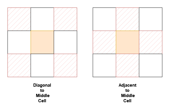
🧩 Approach

Use a lookup table (hash map) to store the coordinates of each value in the grid for O(1) access. For both adjacentSum and diagonalSum, we can define the relative positions of the neighbors and iterate through them to calculate the sum, while ensuring that we stay within the bounds of the grid.

💡 Solution

from typing import List, Tuple

class NeighborSum:

    def __init__(self, grid: List[List[int]]):
        """Initializes the NeighborSum object with the given 2D array grid.

        Args:
            grid (List[List[int]]): The 2D array containing distinct elements.

        Returns:
            None
        """
        self.__grid: List[List[int]] = grid
        self.__R: int = len(grid)
        self.__C: int = len(grid[0])
        self.__lookup: dict[int, Tuple[int, int]] = {}

        for x in range(self.__R):
            for y in range(self.__C):
                self.__lookup[grid[x][y]] = (x, y)


    def adjacentSum(self, value: int) -> int:
        """Returns the sum of elements which are adjacent neighbors of value, that is either to the top, left, right, or bottom of value in grid.

        Args:
            value (int): The value for which to calculate the adjacent sum.

        Returns:
            int: The sum of adjacent neighbors of the given value.
        """
        x, y = self.__lookup[value]

        total: int = 0
        for dx, dy in [(-1, 0), (1, 0), (0, -1), (0, 1)]:
            nx: int = x + dx
            ny: int = y + dy

            if 0 <= nx < self.__R and 0 <= ny < self.__C:
                total += self.__grid[nx][ny]

        return total

    def diagonalSum(self, value: int) -> int:
        """Returns the sum of elements which are diagonal neighbors of value, that is either to the top-left, top-right, bottom-left, or bottom-right of value in grid.

        Args:
            value (int): The value for which to calculate the diagonal sum.

        Returns:
            int: The sum of diagonal neighbors of the given value.
        """
        x, y = self.__lookup[value]

        total: int = 0
        for dx, dy in [(-1, -1), (1, 1), (1, -1), (-1, 1)]:
            nx: int = x + dx
            ny: int = y + dy

            if 0 <= nx < self.__R and 0 <= ny < self.__C:
                total += self.__grid[nx][ny]

        return total

🧮 Complexity Analysis

Time Complexity:
- adjacentSum: O(1) since we only check 4 adjacent neighbors.
- diagonalSum: O(1) since we only check 4 diagonal neighbors.
Space Complexity: O(n^2) for storing the grid and lookup table.

Array / String

13. Roman to Integer
14. Longest Common Prefix
26. Remove Duplicates from Sorted Array
27. Remove Element
28. Find the Index of the First Occurrence in a String
58. Length of Last Word
88. Merge Sorted Array
121. Best Time to Buy and Sell Stock
169. Majority Element
2043. Simple Bank System
2672. Number of Adjacent Elements With the Same Color

13. Roman to Integer

LeetCode Link: Roman to Integer
Difficulty: Easy
Topic(s): Hash Table, String, Math
Company: Google

🧠 Problem Statement

Roman numerals are represented by seven different symbols: I, V, X, L, C, D and M.
Symbol Value
I 1
V 5
X 10
L 50
C 100
D 500
M 1000
For example, 2 is written as II in Roman numeral, just two ones added together. 12 is written as XII, which is simply X + II. The number 27 is written as XXVII, which is XX + V + II.

Roman numerals are usually written largest to smallest from left to right. However, the numeral for four is not IIII. Instead, the number four is written as IV. Because the one is before the five we subtract it making four. The same principle applies to the number nine, which is written as IX. There are six instances where subtraction is used:

I can be placed before V (5) and X (10) to make 4 and 9.

X can be placed before L (50) and C (100) to make 40 and 90.

C can be placed before D (500) and M (1000) to make 400 and 900.

Given a roman numeral, convert it to an integer.

Example 1:
Input: s = "III"
Output: 3
Explanation: III = 3.
Example 2:
Input: s = "LVIII"
Output: 58
Explanation: L = 50, V= 5, III = 3.
Example 3:
Input: s = "MCMXCIV"
Output: 1994
Explanation: M = 1000, CM = 900, XC = 90 and IV = 4.

🧩 Approach

Create a mapping of Roman numeral symbols to their integer values.
Initialize a result variable to 0.
Iterate through the string:
- If the current symbol is less than the next symbol, subtract its value from the result.
- Otherwise, add its value to the result.
Return the result.

💡 Solution

from typing import Dict

class Solution:
    def romanToInt(self, s: str) -> int:
        """
        Convert a Roman numeral to an integer.

        Args:
            s (str): The Roman numeral string.

        Returns:
            int: The integer representation of the Roman numeral.
        """
        romans: Dict[str, int] = {
                "I": 1,
                "V": 5,
                "X": 10,
                "L": 50,
                "C": 100,
                "D": 500,
                "M": 1000
        }
        res: int = 0
        for i in range(len(s)):
            if i + 1 < len(s) and romans[s[i]] < romans[s[i + 1]]:
                res -= romans[s[i]]
            else:
                res += romans[s[i]]
        return res

🧮 Complexity Analysis

Time Complexity: O(n)
Space Complexity: O(1)

14. Longest Common Prefix

LeetCode Link: Longest Common Prefix
Difficulty: Easy
Topic(s): String, Trie
Company: Meta

🧠 Problem Statement

Write a function to find the longest common prefix string amongst an array of strings.

If there is no common prefix, return an empty string "".

Example 1:
Input: strs = ["flower","flow","flight"]
Output: "fl"
Example 2:
Input: strs = ["dog","racecar","car"]
Output: ""
Explanation: There is no common prefix among the input strings.

🧩 Approach

Initialize the result as an empty string.
Iterate through the characters of the first string.
For each character, check if it matches the corresponding character in all other strings.
If a mismatch is found or if the end of any string is reached, return the result.
If all characters match, append the character to the result.
Return the result after checking all characters of the first string.

💡 Solution

from typing import List

class Solution:
    def longestCommonPrefix(self, strs: List[str]) -> str:
        """
        Find the longest common prefix among an array of strings.

        Args:
            strs (List[str]): The list of strings.

        Returns:
            str: The longest common prefix.
        """
        res: str = ""
        for i in range(len(strs[0])):
            for s in strs:
                if i == len(s) or s[i] != strs[0][i]:
                    return res
            res += strs[0][i]
        return res

🧮 Complexity Analysis

Time Complexity: O(n * m)
Space Complexity: O(1)

26. Remove Duplicates from Sorted Array

LeetCode Link: Remove Duplicates from Sorted Array
Difficulty: Easy
Topic(s): Array, Two Pointers
Company: Microsoft

🧠 Problem Statement

Given an integer array nums sorted in non-decreasing order, remove the duplicates in-place such that each unique element appears only once. The relative order of the elements should be kept the same. Then return the number of unique elements in nums.

Consider the number of unique elements of nums to be k, to get accepted, you need to do the following things:

Change the array nums such that the first k elements of nums contain the unique elements in the order they were present in nums initially. The remaining elements of nums are not important as well as the size of nums.

Return k.

Example 1:
Input: nums = [1,1,2]
Output: 2, nums = [1,2,_]
Explanation: Your function should return k = 2, with the first two elements of nums being 1 and 2 respectively.
It does not matter what you leave beyond the returned k (hence they are underscores).
Example 2:
Input: nums = [0,0,1,1,1,2,2,3,3,4]
Output: 5, nums = [0,1,2,3,4,_,_,_,_,_]
Explanation: Your function should return k = 5, with the first five elements of nums being 0, 1, 2, 3, and 4 respectively.
It does not matter what you leave beyond the returned k (hence they are underscores).

🧩 Approach

Use the two-pointer technique:

i: slow pointer, tracks the position of the last unique element.
j: fast pointer, scans the array.

Steps:

Initialize i = 0.
Iterate j from 1 to end of array.
If nums[j] != nums[i], it’s a new unique element:
- Increment i
- Copy nums[j] to nums[i]
After the loop, the first i + 1 elements are the unique values.

💡 Solution

from typing import List

class Solution:
    def removeDuplicates(self, nums: List[int]) -> int:
        """
        Remove duplicates from a sorted array in-place and return the new length.

        Args:
            nums (List[int]): The input sorted array.

        Returns:
            int: The new length of the array after removing duplicates.
        """
        i: int = 0

        for j in range(1, len(nums)):
            if nums[j] != nums[i]:
                i += 1
                nums[i] = nums[j]

        return i + 1

🧮 Complexity Analysis

Time Complexity: O(n)
Space Complexity: O(1)

27. Remove Element

LeetCode Link: Remove Element
Difficulty: Easy
Topic(s): Array, Two Pointers
Company: Apple

🧠 Problem Statement

Given an integer array nums and an integer val, remove all occurrences of val in nums in-place. The order of the elements may be changed. Then return the number of elements in nums that are not equal to val.

Consider the number of elements in nums which are not equal to val be k, to get accepted, you need to do the following things:

Change the array nums such that the first k elements of nums contain the elements which are not equal to val. The remaining elements of nums are not important as well as the size of nums.

Return k.

Example 1:
Input: nums = [3,2,2,3], val = 3
Output: 2, nums = [2,2,_,_]
Explanation: Your function should return k = 2, with the first two elements of nums being 2.
It does not matter what you leave beyond the returned k (hence they are underscores).
Example 2:
Input: nums = [0,1,2,2,3,0,4,2], val = 2
Output: 5, nums = [0,1,4,0,3,_,_,_]
Explanation: Your function should return k = 5, with the first five elements of nums containing 0, 0, 1, 3, and 4.
Note that the five elements can be returned in any order.
It does not matter what you leave beyond the returned k (hence they are underscores).

🧩 Approach

Use the two-pointer technique:

One pointer (i) scans every element.
Another pointer (k) keeps track of the position where the next valid (non-val) element should be placed.

Steps:

Iterate through the array.
If the current element is not equal to val, place it at index k and increment k.
After the loop, k will represent the new length of the array with val removed.

💡 Solution

from typing import List

class Solution:
    def removeElement(self, nums: List[int], val: int) -> int:
        """
        Remove all occurrences of `val` in `nums` in-place and return the new length.

        Args:
            nums (List[int]): The input array.
            val (int): The value to be removed.

        Returns:
            int: The new length of the array after removal.
        """
        k: int = 0
        for i in range(len(nums)):
            if nums[i] != val:
                nums[k] = nums[i]
                k += 1
        return k

🧮 Complexity Analysis

Time Complexity: O(n)
Space Complexity: O(1)

28. Find the Index of the First Occurrence in a String

LeetCode Link: Find the Index of the First Occurrence in a String
Difficulty: Easy
Topic(s): Two Pointers, String, String Matching
Company: Google

🧠 Problem Statement

Given two strings needle and haystack, return the index of the first occurrence of needle in haystack, or -1 if needle is not part of haystack.

Example 1:
Input: haystack = "sadbutsad", needle = "sad"
Output: 0
Explanation: "sad" occurs at index 0 and 6.
The first occurrence is at index 0, so we return 0.
Example 2:
Input: haystack = "leetcode", needle = "leeto"
Output: -1
Explanation: "leeto" did not occur in "leetcode", so we return -1.

🧩 Approach

Use a simple sliding window approach:

Iterate through haystack with a window of size equal to the length of needle.
For each position, check if the substring matches needle.
If a match is found, return the starting index.
If no match is found after checking all possible positions, return -1.

💡 Solution

class Solution:
    def strStr(self, haystack: str, needle: str) -> int:
        """
        Find the index of the first occurrence of `needle` in `haystack`.

        Args:
            haystack (str): The string to search in.
            needle (str): The substring to search for.

        Returns:
            int: The index of the first occurrence of `needle` in `haystack`, or -1 if not found.
        """
        for i in range(len(haystack) + 1 - len(needle)):
            if haystack[i: i + len(needle)] == needle:
                return i
        return -1

🧮 Complexity Analysis

Time Complexity: O(n * m)
Space Complexity: O(1)

58. Length of Last Word

LeetCode Link: Length of Last Word
Difficulty: Easy
Topic(s): String, String Manipulation
Company: Amazon

🧠 Problem Statement

Given a string s consisting of words and spaces, return the length of the last word in the string.

A word is a maximal substring consisting of non-space characters only.

Example 1:
Input: s = "Hello World"
Output: 5
Explanation: The last word is "World" with length 5.
Example 2:
Input: s = "   fly me   to   the moon  "
Output: 4
Explanation: The last word is "moon" with length 4.
Example 3:
Input: s = "luffy is still joyboy"
Output: 6
Explanation: The last word is "joyboy" with length 6.

🧩 Approach

Split the string s into words using the split() method, which automatically handles multiple spaces.
Return the length of the last word in the list of words.

💡 Solution

from typing import List

class Solution:
    def lengthOfLastWord(self, s: str) -> int:
        """
        Calculate the length of the last word in a string.

        Args:
            s (str): The input string.

        Returns:
            int: The length of the last word.
        """
        words: List[str] = s.split()
        return len(words[-1])

🧮 Complexity Analysis

Time Complexity: O(n)
Space Complexity: O(n)

88. Merge Sorted Array

LeetCode Link: Merge Sorted Array
Difficulty: Easy
Topic(s): Array, Two Pointers, Sorting
Company: Meta

🧠 Problem Statement

You are given two integer arrays nums1 and nums2, sorted in non-decreasing order, and two integers m and n, representing the number of elements in nums1 and nums2 respectively.

Merge nums1 and nums2 into a single array sorted in non-decreasing order.

The final sorted array should not be returned by the function, but instead be stored inside the array nums1. To accommodate this, nums1 has a length of m + n, where the first m elements denote the elements that should be merged, and the last n elements are set to 0 and should be ignored. nums2 has a length of n.

Example 1:
Input: nums1 = [1,2,3,0,0,0], m = 3, nums2 = [2,5,6], n = 3
Output: [1,2,2,3,5,6]
Explanation: The arrays we are merging are [1,2,3] and [2,5,6].
The result of the merge is [1,2,2,3,5,6] with the underlined elements coming from nums1.
Example 2:
Input: nums1 = [1], m = 1, nums2 = [], n = 0
Output: [1]
Explanation: The arrays we are merging are [1] and [].
The result of the merge is [1].
Example 3:
Input: nums1 = [0], m = 0, nums2 = [1], n = 1
Output: [1]
Explanation: The arrays we are merging are [] and [1].
The result of the merge is [1].
Note that because m = 0, there are no elements in nums1. The 0 is only there to ensure the merge result can fit in nums1.

🧩 Approach

Use three pointers:

midx points to the last valid element in nums1 (m - 1)
nidx points to the last element in nums2 (n - 1)
right points to the last index in nums1 (m + n - 1)

Compare elements from the back and place the larger one at index right. Decrement pointers accordingly.

Repeat until nidx reaches 0 (no need to worry about midx, since the rest are already in place).

💡 Solution

from typing import List

class Solution:
    def merge(self, nums1: List[int], m: int, nums2: List[int], n: int) -> None:
        """
        Merge two sorted arrays `nums1` and `nums2` into `nums1` in-place.

        Args:
            nums1 (List[int]): The first sorted array with enough space to hold the elements of `nums2`.
            m (int): The number of elements in `nums1`.
            nums2 (List[int]): The second sorted array.
            n (int): The number of elements in `nums2`.

        Returns:
            None: The result is stored in `nums1`.
        """
        midx: int = m - 1
        nidx: int = n - 1
        right: int = m + n - 1

        while nidx >= 0:
            if midx >= 0 and nums1[midx] > nums2[nidx]:
                nums1[right] = nums1[midx]
                midx -= 1
            else:
                nums1[right] = nums2[nidx]
                nidx -= 1

            right -= 1

🧮 Complexity Analysis

Time Complexity: O(m + n)
Space Complexity: O(1)

121. Best Time to Buy and Sell Stock

LeetCode Link: Best Time to Buy and Sell Stock
Difficulty: Easy
Topic(s): Array, Dynamic Programming
Company: Amazon

🧠 Problem Statement

You are given an array prices where prices[i] is the price of a given stock on the ith day.

You want to maximize your profit by choosing a single day to buy one stock and choosing a different day in the future to sell that stock.

Return the maximum profit you can achieve from this transaction. If you cannot achieve any profit, return 0.

Example 1:
Input: prices = [7,1,5,3,6,4]
Output: 5
Explanation: Buy on day 2 (price = 1) and sell on day 5 (price = 6), profit = 6-1 = 5.
Note that buying on day 2 and selling on day 1 is not allowed because you must buy before you sell.
Example 2:
Input: prices = [7,6,4,3,1]
Output: 0
Explanation: In this case, no transactions are done and the max profit = 0.

🧩 Approach

Dynamic programming approach:

Initialize profit to 0 and lowest to the first price.
Iterate through the prices:
- For each price, calculate the potential profit by subtracting lowest from the current price.
- Update profit if the calculated profit is greater than the current profit.
- Update lowest to be the minimum of the current price and lowest.
Return the profit.

This approach ensures that we always consider the lowest price seen so far, allowing us to calculate the maximum profit efficiently.

💡 Solution

from typing import List

class Solution:
    def maxProfit(self, prices: List[int]) -> int:
        """
        Calculate the maximum profit from a single buy and sell transaction.

        Args:
            prices (List[int]): The list of stock prices.

        Returns:
            int: The maximum profit achievable, or 0 if no profit can be made.
        """
        profit: int = 0
        lowest: int = prices[0]

        for price in prices:
            profit = max(profit, price - lowest)
            lowest = min(lowest, price)
        return profit

🧮 Complexity Analysis

Time Complexity: O(n)
Space Complexity: O(1)

169. Majority Element

LeetCode Link: Majority Element
Difficulty: Easy
Topic(s): Array, Hash Table, Divide and Conquer, Counting
Company: Apple

🧠 Problem Statement

Given an array nums of size n, return the majority element.

The majority element is the element that appears more than ⌊n / 2⌋ times. You may assume that the majority element always exists in the array.

Example 1:
Input: nums = [3,2,3]
Output: 3
Example 2:
Input: nums = [2,2,1,1,1,2,2]
Output: 2

🧩 Approach

Boyer-Moore Voting Algorithm:

Initialize a count = 0 and candidate = None.
Iterate through the array:
- If count == 0, set candidate = current element
- If current element == candidate, increment count
- Else, decrement count
At the end, candidate is the majority element.

This works because the majority element appears more than all others combined.

💡 Solution

from typing import List

class Solution:
    def majorityElement(self, nums: List[int]) -> int:
        """
        Find the majority element in an array using Boyer-Moore Voting Algorithm.

        Args:
            nums (List[int]): The input array.

        Returns:
            int: The majority element.
        """
        count: int = 0
        candidate: int = 0

        for num in nums:
            if count == 0:
                candidate = num

            if num == candidate:
                count += 1
            else:
                count -= 1

        return candidate

🧮 Complexity Analysis

Time Complexity: O(n)
Space Complexity: O(1)

2043. Simple Bank System

LeetCode Link: Simple Bank System
Difficulty: Medium
Topic(s): Design, Array
Company: Capital One

🧠 Problem Statement

You have been tasked with writing a program for a popular bank that will automate all its incoming transactions (transfer, deposit, and withdraw). The bank has n accounts numbered from 1 to n. The initial balance of each account is stored in a 0-indexed integer array balance, with the (i + 1)th account having an initial balance of balance[i].

Execute all the valid transactions. A transaction is valid if:

The given account number(s) are between 1 and n, and
The amount of money withdrawn or transferred from is less than or equal to the balance of the account.

Implement the Bank class:

Bank(long[] balance) Initializes the object with the 0-indexed integer array balance.
boolean transfer(int account1, int account2, long money) Transfers money dollars from the account numbered account1 to the account numbered account2. Return true if the transaction was successful, false otherwise.
boolean deposit(int account, long money) Deposit money dollars into the account numbered account. Return true if the transaction was successful, false otherwise.
boolean withdraw(int account, long money) Withdraw money dollars from the account numbered account. Return true if the transaction was successful, false otherwise.

Example 1:

Input
["Bank", "withdraw", "transfer", "deposit", "transfer", "withdraw"]
[[[10, 100, 20, 50, 30]], [3, 10], [5, 1, 20], [5, 20], [3, 4, 15], [10, 50]]
Output
[null, true, true, true, false, false]

Explanation
Bank bank = new Bank([10, 100, 20, 50, 30]);
bank.withdraw(3, 10);    // return true, account 3 has a balance of $20, so it is valid to withdraw $10.
                         // Account 3 has $20 - $10 = $10.
bank.transfer(5, 1, 20); // return true, account 5 has a balance of $30, so it is valid to transfer $20.
                         // Account 5 has $30 - $20 = $10, and account 1 has $10 + $20 = $30.
bank.deposit(5, 20);     // return true, it is valid to deposit $20 to account 5.
                         // Account 5 has $10 + $20 = $30.
bank.transfer(3, 4, 15); // return false, the current balance of account 3 is $10,
                         // so it is invalid to transfer $15 from it.
bank.withdraw(10, 50);   // return false, it is invalid because account 10 does not exist.

🧩 Approach

Initialize the Bank class with the given balances.
Implement the transfer method to check for valid accounts and sufficient balance before transferring money.
Implement the deposit method to add money to the specified account if valid.
Implement the withdraw method to deduct money from the specified account if valid.

💡 Solution

from typing import List

class Bank:

    def __init__(self, balance: List[int]):
        """
        Initialize the Bank with the given balances.

        Args:
            balance (List[int]): The initial balances of the accounts.
        """
        self.balance: List[int] = balance

    def transfer(self, account1: int, account2: int, money: int) -> bool:
        """
        Transfer money from account1 to account2 if valid.

        Args:
            account1 (int): The account number to transfer money from.
            account2 (int): The account number to transfer money to.
            money (int): The amount of money to transfer.

        Returns:
            bool: True if the transfer was successful, False otherwise.
        """
        if (
            account1 > len(self.balance)
            or account2 > len(self.balance)
            or self.balance[account1 - 1] < money
        ):
            return False
        self.balance[account1 - 1] -= money
        self.balance[account2 - 1] += money
        return True

    def deposit(self, account: int, money: int) -> bool:
        """
        Deposit money into the specified account if valid.

        Args:
            account (int): The account number to deposit money into.
            money (int): The amount of money to deposit.

        Returns:
            bool: True if the deposit was successful, False otherwise.
        """
        if account > len(self.balance):
            return False

        self.balance[account - 1] += money
        return True

    def withdraw(self, account: int, money: int) -> bool:
        """
        Withdraw money from the specified account if valid.

        Args:
            account (int): The account number to withdraw money from.
            money (int): The amount of money to withdraw.

        Returns:
            bool: True if the withdrawal was successful, False otherwise.
        """
        if account > len(self.balance) or self.balance[account - 1] < money:
            return False

        self.balance[account - 1] -= money
        return True

🧮 Complexity Analysis

Time Complexity: O(1)
Space Complexity: O(1)

2672. Number of Adjacent Elements With the Same Color

LeetCode Link: Number of Adjacent Elements With the Same Color
Difficulty: Easy
Topic(s): Array, Simulation
Company: Capital One

🧠 Problem Statement

You are given an integer n representing an array colors of length n where all elements are set to 0’s meaning uncolored. You are also given a 2D integer array queries where queries[i] = [indexi, colori]. For the ith query:

Set colors[indexi] to colori. Count the number of adjacent pairs in colors which have the same color (regardless of colori). Return an array answer of the same length as queries where answer[i] is the answer to the ith query.

Example 1:
Input: n = 4, queries = [[0,2],[1,2],[3,1],[1,1],[2,1]]

Output: [0,1,1,0,2]

Explanation:

Initially array colors = [0,0,0,0], where 0 denotes uncolored elements of the array.
After the 1st query colors = [2,0,0,0]. The count of adjacent pairs with the same color is 0.
After the 2nd query colors = [2,2,0,0]. The count of adjacent pairs with the same color is 1.
After the 3rd query colors = [2,2,0,1]. The count of adjacent pairs with the same color is 1.
After the 4th query colors = [2,1,0,1]. The count of adjacent pairs with the same color is 0.
After the 5th query colors = [2,1,1,1]. The count of adjacent pairs with the same color is 2.
Example 2:
Input: n = 1, queries = [[0,100000]]

Output: [0]

Explanation:

After the 1st query colors = [100000]. The count of adjacent pairs with the same color is 0.

🧩 Approach

Initialize a count variable to keep track of adjacent pairs with the same color.
Create an array nums of size n initialized to 0 to represent uncolored elements.
For each query:
- Check the previous and next elements of the index being colored.
- If the current element is already colored and matches the previous or next element, decrement the count.
- Update the color of the current index.
- If the new color matches the previous or next element, increment the count.
Append the current count to the result list after each query.

💡 Solution

from typing import List

class Solution:
    def colorTheArray(self, n: int, queries: List[List[int]]) -> List[int]:
        count: int = 0
        res: List[int] = []
        nums: List[int] = [0 for _ in range(n)]

        for idx, color in queries:
            prev: int = nums[idx - 1] if idx > 0 else 0
            nxt: int = nums[idx + 1] if idx < n - 1 else 0

            if nums[idx] and nums[idx] == prev:
                count -= 1

            if nums[idx] and nums[idx] == nxt:
                count -= 1

            nums[idx] = color

            if nums[idx] and nums[idx] == prev:
                count += 1

            if nums[idx] and nums[idx] == nxt:
                count += 1

            res.append(count)

        return res

🧮 Complexity Analysis

Time Complexity: O(n)
Space Complexity: O(n)

Two Pointers

125. Valid Palindrome
392. Is Subsequence

125. Valid Palindrome

LeetCode Link: Valid Palindrome
Difficulty: Easy
Topics: String, Two Pointers
Company: Meta

🧠 Problem Statement

A phrase is a palindrome if, after converting all uppercase letters into lowercase letters and removing all non-alphanumeric characters, it reads the same forward and backward. Alphanumeric characters include letters and numbers.

Given a string s, return true if it is a palindrome, or false otherwise.

Example 1:
Input: s = "A man, a plan, a canal: Panama"
Output: true
Explanation: "amanaplanacanalpanama" is a palindrome.
Example 2:
Input: s = "race a car"
Output: false
Explanation: "raceacar" is not a palindrome.
Example 3:
Input: s = " "
Output: true
Explanation: s is an empty string "" after removing non-alphanumeric characters.
Since an empty string reads the same forward and backward, it is a palindrome.

🧩 Approach

Use the Two Pointers approach:

Initialize two pointers, l at the start and r at the end of the string.
Move the left pointer l to the right until it points to an alphanumeric character.
Move the right pointer r to the left until it points to an alphanumeric character.
Compare the characters at l and r after converting them to lowercase.
If they are not equal, return False.
Move both pointers inward (l to the right and r to the left) and repeat steps 2-5 until the pointers meet or cross.
If all characters match, return True.

💡 Solution

class Solution:
    def isPalindrome(self, s: str) -> bool:
        """
        Check if the given string is a palindrome after removing non-alphanumeric characters
        and converting to lowercase.

        Args:
            s (str): The input string to check.

        Returns:
            bool: True if the string is a palindrome, False otherwise.
        """
        l: int = 0
        r: int = len(s) - 1

        while l < r:
            while l < r and not self.isalnum(s[l]):
                l += 1
            while r > l and not self.isalnum(s[r]):
                r -= 1
            if s[l].lower() != s[r].lower():
                return False
            l, r = l + 1, r - 1

        return True

    def isalnum(self, c: str):
        """
        Check if the character is alphanumeric.

        Args:
            c (str): The character to check.

        Returns:
            bool: True if the character is alphanumeric, False otherwise.
        """
        return (
            ord("A") <= ord(c) <= ord("Z")
            or ord("a") <= ord(c) <= ord("z")
            or ord("0") <= ord(c) <= ord("9")
        )

🧮 Complexity Analysis

Time Complexity: O(n)
Space Complexity: O(1)

392. Is Subsequence

LeetCode Link: Is Subsequence
Difficulty: Easy
Topics: String, Two Pointers
Company: Uber

🧠 Problem Statement

Given two strings s and t, return true if s is a subsequence of t, or false otherwise.

A subsequence of a string is a new string that is formed from the original string by deleting some (can be none) of the characters without disturbing the relative positions of the remaining characters. (i.e., "ace" is a subsequence of "abcde" while "aec" is not).

Example 1:
Input: s = "abc", t = "ahbgdc"
Output: true
Example 2:
Input: s = "axc", t = "ahbgdc"
Output: false

🧩 Approach

Use the Two Pointers approach:

Initialize two pointers, i for string s and j for string t.
Iterate through both strings:
- If the characters at s[i] and t[j] match, move the pointer i to the next character in s.
- Always move the pointer j to the next character in t.
If the pointer i reaches the end of s, it means all characters of s were found in t in order, so return True.
If the loop ends and i has not reached the end of s, return False.

💡 Solution

class Solution:
    def isSubsequence(self, s: str, t: str) -> bool:
        """
        Check if string `s` is a subsequence of string `t`.

        Args:
            s (str): The string to check as a subsequence.
            t (str): The string in which to check for the subsequence.

        Returns:
            bool: True if `s` is a subsequence of `t`, False otherwise.
        """
        i: int = 0
        j: int = 0

        while i < len(s) and j < len(t):
            if s[i] == t[j]:
                i += 1
            j += 1

        return True if i == len(s) else False

🧮 Complexity Analysis

Time Complexity: O(n)
Space Complexity: O(1)

Hashmap

1. Two Sum
202. Happy Number
205. Isomorphic Strings
219. Contains Duplicate II
242. Valid Anagram
290. Word Pattern
383 Ransom Note

1. Two Sum

LeetCode Link: Two Sum
Difficulty: Easy
Topics: Array, Hash Table
Company: Google

🧠 Problem Statement

Given an array of integers nums and an integer target, return indices of the two numbers such that they add up to target.

You may assume that each input would have exactly one solution, and you may not use the same element twice.

You can return the answer in any order.

Example 1:
Input: nums = [2,7,11,15], target = 9
Output: [0,1]
Explanation: Because nums[0] + nums[1] == 9, we return [0, 1].
Example 2:
Input: nums = [3,2,4], target = 6
Output: [1,2]
Example 3:
Input: nums = [3,3], target = 6
Output: [0,1]

🧩 Approach

Create a hashmap (dictionary) to store the indices of the numbers in nums.
Iterate through the nums array:
- For each number, calculate the complement (target - nums[i]).
- Check if the complement exists in the hashmap:
  - If it does, return the current index and the index of the complement.
  - If it doesn’t, add the current number and its index to the hashmap.
If no solution is found, return an empty list (though the problem guarantees a solution).

💡 Solution

from typing import List, Dict

class Solution:
    def twoSum(self, nums: List[int], target: int) -> List[int]:
        """
        Find indices of two numbers in nums that add up to target.

        Args:
            nums (List[int]): List of integers.
            target (int): Target sum.

        Returns:
            List[int]: Indices of the two numbers that add up to target.
        """
        h: Dict[int, int] = {}

        for i in range(len(nums)):
            h[nums[i]] = i

        for i in range(len(nums)):
            y: int = target - nums[i]

            if y in h and h[y] != i:
                return [i, h[y]]

🧮 Complexity Analysis

Time Complexity: O(n)
Space Complexity: O(n)

202. Happy Number

LeetCode Link: Happy Number
Difficulty: Easy
Topics: Hash Table, Math, Two Pointers
Company: Google

🧠 Problem Statement

Write an algorithm to determine if a number n is happy.

A happy number is a number defined by the following process:

Starting with any positive integer, replace the number by the sum of the squares of its digits. Repeat the process until the number equals 1 (where it will stay), or it loops endlessly in a cycle which does not include 1. Those numbers for which this process ends in 1 are happy. Return true if n is a happy number, and false if not.

Example 1:
Input: n = 19
Output: true
Explanation:
12 + 92 = 82
82 + 22 = 68
62 + 82 = 100
12 + 02 + 02 = 1
Example 2:
Input: n = 2
Output: false

🧩 Approach

Use a hashset to track seen numbers:

Initialize an empty set to keep track of numbers that have been seen.
Convert the number n to a string to easily access its digits.
While the current number is not in the seen set:
- Add the current number to the seen set.
- Calculate the sum of the squares of its digits.
- If the sum equals 1, return True.
- Update the current number to this new sum.
If the current number is already in the seen set, return False (indicating a cycle).

💡 Solution

from typing import Set

class Solution:
    def isHappy(self, n: int) -> bool:
        """
        Determine if a number n is a happy number.

        Args:
            n (int): The number to check.

        Returns:
            bool: True if n is a happy number, False otherwise.
        """
        seen: Set[str] = set()
        cur: str = str(n)

        while cur not in seen:
            seen.add(cur)
            total: int = 0

            for digit in cur:
                digit = int(digit)
                total += digit**2

            if total == 1:
                return True

            cur = str(total)

        return False

🧮 Complexity Analysis

Time Complexity: O(log n)
Space Complexity: O(log n)

205. Isomorphic Strings

LeetCode Link: Isomorphic Strings
Difficulty: Easy
Topics: Hash Table, String
Company: Meta

🧠 Problem Statement

Given two strings s and t, determine if they are isomorphic.

Two strings s and t are isomorphic if the characters in s can be replaced to get t.

All occurrences of a character must be replaced with another character while preserving the order of characters. No two characters may map to the same character, but a character may map to itself.

Example 1:
Input: s = "egg", t = "add"

Output: true

Explanation:

The strings s and t can be made identical by:

Mapping 'e' to 'a'.
Mapping 'g' to 'd'.
Example 2:
Input: s = "foo", t = "bar"

Output: false

Explanation:

The strings s and t can not be made identical as 'o' needs to be mapped to both 'a' and 'r'.
Example 3:
Input: s = "paper", t = "title"

Output: true

🧩 Approach

Use hashmaps:

Create two hashmaps (dictionaries) to map characters from s to t and from t to s.
Iterate through the characters of both strings simultaneously:
- For each character pair (c1, c2) from s and t:
  - Check if c1 is already mapped to a different character than c2 or if c2 is already mapped to a different character than c1.
  - If either condition is true, return False.
  - Otherwise, update the mappings for c1 to c2 and c2 to c1.
If all character pairs are processed without conflicts, return True.

💡 Solution

from typing import Dict

class Solution:
    def isIsomorphic(self, s: str, t: str) -> bool:
        """
        Check if two strings s and t are isomorphic.

        Args:
            s (str): First string.
            t (str): Second string.

        Returns:
            bool: True if s and t are isomorphic, False otherwise.
        """
        map_st: Dict[str, str] = {}
        map_ts: Dict[str, str] = {}

        for c1, c2 in zip(s, t):
            if (c1 in map_st and map_st[c1] != c2) or (
                c2 in map_ts and map_ts[c2] != c1
            ):
                return False

            map_st[c1] = c2
            map_ts[c2] = c1

        return True

🧮 Complexity Analysis

Time Complexity: O(n)
Space Complexity: O(n)

219. Contains Duplicate II

LeetCode Link: Contains Duplicate II
Difficulty: Easy
Topics: Array, Hash Table
Company: Meta

🧠 Problem Statement

Given an integer array nums and an integer k, return true if there are two distinct indices i and j in the array such that nums[i] == nums[j] and abs(i - j) <= k.

Example 1:
Input: nums = [1,2,3,1], k = 3
Output: true
Example 2:
Input: nums = [1,0,1,1], k = 1
Output: true
Example 3:
Input: nums = [1,2,3,1,2,3], k = 2
Output: false

🧩 Approach

Use a hashmap to track the last seen index of each number:

Create an empty hashmap (dictionary) to store the last seen index of each number.
Iterate through the array with both index and value:
- For each number, check if it exists in the hashmap:
  - If it does, check if the absolute difference between the current index and the last seen index is less than or equal to k. If true, return True.
- Update the hashmap with the current index for the number.
If no such pair is found, return False.

💡 Solution

from typing import Dict

class Solution:
    def containsNearbyDuplicate(self, nums: List[int], k: int) -> bool:
        """
        Check if there are two distinct indices i and j such that nums[i] == nums[j] and abs(i - j) <= k.

        Args:
            nums (List[int]): List of integers.
            k (int): Maximum allowed index difference.
        Returns:
            bool: True if such indices exist, False otherwise.
        """
        hset: Dict[int, int] = {}

        for i, num in enumerate(nums):
            if num in hset and abs(i - hset[num]) <= k:
                return True
            hset[num] = i

        return False

🧮 Complexity Analysis

Time Complexity: O(n)
Space Complexity: O(n)

242. Valid Anagram

LeetCode Link: Valid Anagram
Difficulty: Easy
Topics: Hash Table, String, Sorting
Company: Google

🧠 Problem Statement

Given two strings s and t, return true if t is an anagram of s, and false otherwise.

Example 1:
Input: s = "anagram", t = "nagaram"

Output: true
Example 2:
Input: s = "rat", t = "car"

Output: false

🧩 Approach

Use hashmaps:

Check if the lengths of s and t are equal. If not, return False.
Create two hashmaps (dictionaries) to count the occurrences of each character in s and t.
Iterate through the characters in both strings:
- For each character in s, increment its count in s_counter.
- For each character in t, increment its count in t_counter.
Compare the two hashmaps:
- If they are equal, return True.
- If they differ, return False.

💡 Solution

from typing import Dict

class Solution:
    def isAnagram(self, s: str, t: str) -> bool:
        """
        Check if two strings s and t are anagrams of each other.

        Args:
            s (str): First string.
            t (str): Second string.

        Returns:
            bool: True if s and t are anagrams, False otherwise.
        """
        if len(s) != len(t):
            return False

        s_counter: Dict[str, int] = {}
        t_counter: Dict[str, int] = {}

        for i in range(len(s)):
            s_counter[s[i]] = 1 + s_counter.get(s[i], 0)
            t_counter[t[i]] = 1 + t_counter.get(t[i], 0)

        for c in s_counter:
            if s_counter[c] != t_counter.get(c, 0):
                return False

        return True

🧮 Complexity Analysis

Time Complexity: O(n)
Space Complexity: O(n)

290. Word Pattern

LeetCode Link: Word Pattern
Difficulty: Easy
Topics: Hash Table, String
Company: Amazon

🧠 Problem Statement

Given a pattern and a string s, find if s follows the same pattern.

Here follow means a full match, such that there is a bijection between a letter in pattern and a non-empty word in s. Specifically:

Each letter in pattern maps to exactly one unique word in s. Each unique word in s maps to exactly one letter in pattern. No two letters map to the same word, and no two words map to the same letter.

Example 1:
Input: pattern = "abba", s = "dog cat cat dog"

Output: true

Explanation:

The bijection can be established as:

'a' maps to "dog".
'b' maps to "cat".
Example 2:
Input: pattern = "abba", s = "dog cat cat fish"

Output: false
Example 3:
Input: pattern = "aaaa", s = "dog cat cat dog"

Output: false

🧩 Approach

Use hashmaps:

Split the string s into words.
Check if the length of words matches the length of pattern. If not, return False.
Create two hashmaps:
- map_pw: Maps characters in pattern to words in s.
- map_wp: Maps words in s to characters in pattern.
Iterate through the characters in pattern and the corresponding words in s:
- For each character c1 in pattern and word c2
  - Check if c1 is already mapped to a different word than c2 or if c2 is already mapped to a different character than c1.
  - If either condition is true, return False.
  - Otherwise, update the mappings for c1 to c2 and c2 to c1.
If all character-word pairs are processed without conflicts, return True.

💡 Solution

from typing import List, Dict

class Solution:
    def wordPattern(self, pattern: str, s: str) -> bool:
        """
        Check if the string s follows the same pattern as the given pattern.

        Args:
            pattern (str): The pattern string.
            s (str): The string to check against the pattern.

        Returns:
            bool: True if s follows the pattern, False otherwise.
        """
        words: List[str] = s.split()

        map_pw: Dict[str, str] = {}
        map_wp: Dict[str, str] = {}

        if len(words) != len(pattern):
            return False

        for c1, c2 in zip(pattern, words):
            if (c1 in map_pw and map_pw[c1] != c2) or (
                c2 in map_wp and map_wp[c2] != c1
            ):
                return False

            map_pw[c1] = c2
            map_wp[c2] = c1

        return True

🧮 Complexity Analysis

Time Complexity: O(n)
Space Complexity: O(n)

383. Ransom Note

LeetCode Link: Ransom Note
Difficulty: Easy
Topics: Hash Table, String, Counting
Company: Adobe

🧠 Problem Statement

Given two strings ransomNote and magazine, return true if ransomNote can be constructed by using the letters from magazine and false otherwise.

Each letter in magazine can only be used once in ransomNote.

Example 1:
Input: ransomNote = "a", magazine = "b"
Output: false
Example 2:
Input: ransomNote = "aa", magazine = "ab"
Output: false
Example 3:
Input: ransomNote = "aa", magazine = "aab"
Output: true

🧩 Approach

Use a hashmap (dictionary) to count the occurrences of each character in the magazine.
Iterate through each character in the ransomNote:
- If the character is not in the hashmap, return False.
- If the character’s count is 1, remove it from the hashmap.
- If the character’s count is greater than 1, decrement its count in the hashmap.
If all characters in the ransomNote can be matched with those in the magazine, return True.

💡 Solution

from typing import Dict

class Solution:
    def canConstruct(self, ransomNote: str, magazine: str) -> bool:
        """
        Check if ransomNote can be constructed from magazine using character counts.

        Args:
            ransomNote (str): The string to be constructed.
            magazine (str): The string from which characters can be used.

        Returns:
            bool: True if ransomNote can be constructed from magazine, False otherwise.
        """
        counter: Dict[str, int] = {}
        for c in magazine:
            if c in counter:
                counter[c] += 1
            else:
                counter[c] = 1

        for c in ransomNote:
            if c not in counter:
                return False
            elif counter[c] == 1:
                del counter[c]
            else:
                counter[c] -= 1

        return True

🧮 Complexity Analysis

Time Complexity: O(n + m)
Space Complexity: O(n)

Intervals

228. Summary Ranges

228. Summary Ranges

LeetCode Link: Summary Ranges
Difficulty: Easy
Topics: Array
Company: Google

🧠 Problem Statement

You are given a sorted unique integer array nums.

A range [a,b] is the set of all integers from a to b (inclusive).

Return the smallest sorted list of ranges that cover all the numbers in the array exactly. That is, each element of nums is covered by exactly one of the ranges, and there is no integer x such that x is in one of the ranges but not in nums.

Each range [a,b] in the list should be output as:

“a->b” if a != b “a” if a == b

Example 1:
Input: nums = [0,1,2,4,5,7]
Output: ["0->2","4->5","7"]
Explanation: The ranges are:
[0,2] --> "0->2"
[4,5] --> "4->5"
[7,7] --> "7"
Example 2:
Input: nums = [0,2,3,4,6,8,9]
Output: ["0","2->4","6","8->9"]
Explanation: The ranges are:
[0,0] --> "0"
[2,4] --> "2->4"
[6,6] --> "6"
[8,9] --> "8->9"

🧩 Approach

To solve the problem of summarizing ranges in a sorted unique integer array, we can use a straightforward approach by iterating through the array and identifying consecutive sequences of numbers. Here’s a step-by-step breakdown of the approach:

Initialization: Start by initializing an empty list to store the resulting ranges and a variable to keep track of the starting number of the current range.
Iterate through the array: Loop through the array using an index. For each number, check if it is the start of a new range or part of an existing range.
Identify ranges: If the current number is consecutive to the previous number (i.e., nums[i] == nums[i-1] + 1), continue to the next number. If not, it means the current range has ended.
Store the range: When a range ends, check if the start and end of the range are the same. If they are, add just the start number to the result list. If they are different, add the range in the format “start->end”.
Handle the last range: After the loop, ensure to add the last identified range to the result list.
Return the result: Finally, return the list of summarized ranges.

💡 Solution

class Solution:
    def summaryRanges(self, nums: List[int]) -> List[str]:
        """
        Summarize ranges in a sorted unique integer array.

        Args:
            nums (List[int]): A sorted unique integer array.

        Returns:
            List[str]: A list of summarized ranges.
        """
        ans: List[str] = []
        i: int = 0

        while i < len(nums):
            start: int = nums[i]

            while i < len(nums) - 1 and nums[i] + 1 == nums[i + 1]:
                i += 1

            if start != nums[i]:
                ans.append(str(start) + "->" + str(nums[i]))
            else:
                ans.append(str(nums[i]))

            i += 1

        return ans

🧮 Complexity Analysis

Time Complexity: O(n)
Space Complexity: O(n)

Stack

20. Valid Parentheses

20. Valid Parentheses

LeetCode Link: Valid Parentheses
Difficulty: Easy
Topics: String, Stack
Company: Meta

🧠 Problem Statement

Given a string s containing just the characters '(', ')', '{', '}', '[' and ']', determine if the input string is valid.

An input string is valid if:

Open brackets must be closed by the same type of brackets.

Open brackets must be closed in the correct order.

Every close bracket has a corresponding open bracket of the same type.

Example 1:
Input: s = "()"

Output: true
Example 2:
Input: s = "()[]{}"

Output: true
Example 3:
Input: s = "(]"

Output: false
Example 4:
Input: s = "([])"

Output: true
Example 5:
Input: s = "([)]"

Output: false

🧩 Approach

To solve the problem of validating parentheses, we can use a stack data structure. The idea is to iterate through each character in the string and perform the following steps:

Push Open Brackets: If the character is an opening bracket ('(', '{', '['), we push it onto the stack.
Check Close Brackets: If the character is a closing bracket (')', '}', ']'), we check if the stack is empty. If it is empty, it means there is no corresponding opening bracket, and we return False. If the stack is not empty, we pop the top element from the stack and check if it matches the corresponding opening bracket. If it does not match, we return False.
Final Check: After processing all characters, if the stack is empty, it means all opening brackets had matching closing brackets in the correct order, and we return True. If the stack is not empty, we return False.

💡 Solution

from typing import Dict

class Solution:
    def isValid(self, s: str) -> bool:
        """
        Determine if the input string of parentheses is valid.

        Args:
            s (str): The input string containing parentheses.

        Returns:
            bool: True if the string is valid, False otherwise.
        """
        hashmap: Dict[str, str] = {")": "(", "]": "[", "}": "{"}
        stack: List[str] = []

        for c in s:
            if c not in hashmap:
                stack.append(c)
            else:
                if not stack:
                    return False
                else:
                    popped = stack.pop()
                    if popped != hashmap[c]:
                        return False

        return not stack

🧮 Complexity Analysis

Time Complexity: O(n)
Space Complexity: O(n)

Linked List

21. Merge Two Sorted Lists
141. Linked List Cycle

21. Merge Two Sorted Lists

LeetCode Link: Merge Two Sorted Lists
Difficulty: Easy
Topics: Linked List, Recursion
Company: Microsoft

🧠 Problem Statement

You are given the heads of two sorted linked lists list1 and list2.

Merge the two lists into one sorted list. The list should be made by splicing together the nodes of the first two lists.

Return the head of the merged linked list.

Example 1:
Input: list1 = [1,2,4], list2 = [1,3,4]
Output: [1,1,2,3,4,4]
Example 2:
Input: list1 = [], list2 = []
Output: []
Example 3:
Input: list1 = [], list2 = [0]
Output: [0]

🧩 Approach

To merge two sorted linked lists, we can use a two-pointer technique to traverse both lists and build a new sorted list. Here are the steps:

Initialization: Create a dummy node to serve as the starting point of the merged list. This helps simplify edge cases. Also, create a pointer cur that will point to the current node in the merged list.
Traversal: Use a while loop to traverse both linked lists until we reach the end of one of them. In each iteration, compare the values of the current nodes of both lists:
- If the value of the current node in list1 is less than that in list2, append the node from list1 to the merged list and move the pointer in list1 to the next node.
- Otherwise, append the node from list2 to the merged list and move the pointer in list2 to the next node.
Appending Remaining Nodes: After the loop, one of the lists may still have remaining nodes. Since both lists are sorted, we can simply append the remaining nodes to the end of the merged list.
Return Result: Finally, return the merged list starting from the node next to the dummy node.

💡 Solution

from typing import Optional

# Definition for singly-linked list.
# class ListNode:
#     def __init__(self, val=0, next=None):
#         self.val = val
#         self.next = next

class Solution:
    def mergeTwoLists(self, list1: Optional[ListNode], list2: Optional[ListNode]) -> Optional[ListNode]:
        """
        Merge two sorted linked lists into one sorted linked list.

        Args:
            list1 (Optional[ListNode]): The head of the first sorted linked list.
            list2 (Optional[ListNode]): The head of the second sorted linked list.

        Returns:
            Optional[ListNode]: The head of the merged sorted linked list.
        """
        dummy: ListNode = ListNode()
        cur: ListNode = dummy

        while list1 and list2:
            if list1.val < list2.val:
                cur.next = list1
                cur = list1
                list1 = list1.next
            else:
                cur.next = list2
                cur = list2
                list2 = list2.next

        cur.next = list1 if list1 else list2

        return dummy.next

🧮 Complexity Analysis

Time Complexity: O(n)
Space Complexity: O(1)

141. Linked List Cycle

LeetCode Link: Linked List Cycle
Difficulty: Easy
Topics: Linked List, Two Pointers
Company: Microsoft

🧠 Problem Statement

Given head, the head of a linked list, determine if the linked list has a cycle in it.

There is a cycle in a linked list if there is some node in the list that can be reached again by continuously following the next pointer. Internally, pos is used to denote the index of the node that tail’s next pointer is connected to. Note that pos is not passed as a parameter.

Return true if there is a cycle in the linked list. Otherwise, return false.

Example 1:
Input: head = [3,2,0,-4], pos = 1
Output: true
Explanation: There is a cycle in the linked list, where the tail connects to the 1st node (0-indexed).
Example 2:
Input: head = [1,2], pos = 0
Output: true
Explanation: There is a cycle in the linked list, where the tail connects to the 0th node.
Example 3:
Input: head = [1], pos = -1
Output: false
Explanation: There is no cycle in the linked list.

🧩 Approach

To determine if a linked list has a cycle, we can use the Floyd’s Cycle-Finding Algorithm, also known as the Tortoise and Hare algorithm. This approach uses two pointers that traverse the linked list at different speeds.

Initialization: We start by creating two pointers, slow and fast. Both pointers are initialized to the head of the linked list.
Traversal: We move the slow pointer one step at a time (i.e., slow = slow.next), while the fast pointer moves two steps at a time (i.e., fast = fast.next.next).
Cycle Detection: If there is a cycle in the linked list, the fast pointer will eventually meet the slow pointer. If the fast pointer reaches the end of the list (i.e., fast or fast.next becomes None), then there is no cycle in the list.
Return Result: If the slow pointer meets the fast pointer, we return True, indicating that there is a cycle. If the fast pointer reaches the end of the list, we return False.

💡 Solution

from typing import Optional

# Definition for singly-linked list.
# class ListNode:
#     def __init__(self, x):
#         self.val = x
#         self.next = None

class Solution:
    def hasCycle(self, head: Optional[ListNode]) -> bool:
        """
        Determine if the linked list has a cycle.

        Args:
            head (Optional[ListNode]): The head of the linked list.

        Returns:
            bool: True if there is a cycle, False otherwise.
        """
        dummy: ListNode = ListNode()
        dummy.next = head
        slow: ListNode = dummy
        fast: ListNode = dummy

        while fast and fast.next:
            fast = fast.next.next
            slow = slow.next

            if slow is fast:
                return True

        return False

🧮 Complexity Analysis

Time Complexity: O(n)
Space Complexity: O(1)

Binary Tree

100. Same Tree
101. Symmetric Tree
104. Maximum Depth of Binary Tree
112. Path Sum
222. Count Complete Tree Nodes
226. Invert Binary Tree
257. Binary Tree Paths
530. Minimum Absolute Difference in BST
637. Average of Levels in Binary Tree

100. Same Tree

LeetCode Link: Same Tree
Difficulty: Easy
Topic(s): Binary Tree, Depth-First Search, Breadth-First Search
Company: Apple

🧠 Problem Statement

Given the roots of two binary trees p and q, write a function to check if they are the same or not.

Two binary trees are considered the same if they are structurally identical, and the nodes have the same value.

Example 1:
Input: p = [1,2,3], q = [1,2,3]
Output: true
Example 2:
Input: p = [1,2], q = [1,null,2]
Output: false
Example 3:
Input: p = [1,2,1], q = [1,1,2]
Output: false

🧩 Approach

DFS (Depth-First Search):
- Recursively compare the nodes of both trees.
- If both nodes are None, they are the same.
- If one node is None and the other is not, they are different.
- If the values of the nodes are different, they are different.
- Recursively check the left and right subtrees.

💡 Solution

from typing import Optional

# Definition for a binary tree node.
# class TreeNode:
#     def __init__(self, val=0, left=None, right=None):
#         self.val = val
#         self.left = left
#         self.right = right


class Solution:
    def isSameTree(self, p: Optional[TreeNode], q: Optional[TreeNode]) -> bool:
        """
        Determine if two binary trees are the same.

        Args:
            p (Optional[TreeNode]): The root node of the first binary tree.
            q (Optional[TreeNode]): The root node of the second binary tree.

        Returns:
            bool: True if the two binary trees are the same, False otherwise.
        """
        def balanced(p: Optional[TreeNode], q: Optional[TreeNode]):
            """
            Helper function to determine if two binary trees are the same.
            Args:
                p (Optional[TreeNode]): The root node of the first binary tree.
                q (Optional[TreeNode]): The root node of the second binary tree.
            Returns:
                bool: True if the two binary trees are the same, False otherwise.
            """
            if not p and not q:
                return True

            if (p and not q) or (q and not p):
                return False

            if p.val != q.val:
                return False

            return balanced(p.left, q.left) and balanced(p.right, q.right)

        return balanced(p, q)

🧮 Complexity Analysis

Time Complexity: O(n + m)
Space Complexity: O(h_p + h_q)

101. Symmetric Tree

LeetCode Link: Symmetric Tree
Difficulty: Easy
Topic(s): Binary Tree, Depth-First Search, Breadth-First Search
Company: Apple

🧠 Problem Statement

Given the root of a binary tree, check whether it is a mirror of itself (i.e., symmetric around its center).

Example 1:
Input: root = [1,2,2,3,4,4,3]
Output: true
Example 2:
Input: root = [1,2,2,null,3,null,3]
Output: false

🧩 Approach

DFS (Depth-First Search):
- Recursively compare the left and right subtrees.
- If both nodes are None, they are symmetric.
- If one node is None and the other is not, they are not symmetric.
- If the values of the nodes are different, they are not symmetric.
- Recursively check the left subtree of one tree with the right subtree of the other tree and vice versa.

💡 Solution

from typing import Optional

# Definition for a binary tree node.
# class TreeNode:
#     def __init__(self, val=0, left=None, right=None):
#         self.val = val
#         self.left = left
#         self.right = right

class Solution:
    def isSymmetric(self, root: Optional[TreeNode]) -> bool:
        """
        Determine if a binary tree is symmetric.

        Args:
            root (Optional[TreeNode]): The root node of the binary tree.

        Returns:
            bool: True if the binary tree is symmetric, False otherwise.
        """
        def same(root1: Optional[TreeNode], root2: Optional[TreeNode]):
            """
            Helper function to determine if a binary tree is symmetric.

            Args:
                root1 (Optional[TreeNode]): The root node of the first subtree.
                root2 (Optional[TreeNode]): The root node of the second subtree.

            Returns:
                bool: True if the binary tree is symmetric, False otherwise.
            """
            if not root1 and not root2:
                return True

            if not root1 or not root2:
                return False

            if root1.val != root2.val:
                return False

            return same(root1.left, root2.right) and same(root1.right, root2.left)

        return same(root, root)

🧮 Complexity Analysis

Time Complexity: O(n + m)
Space Complexity: O(h_p + h_q)

104. Maximum Depth of Binary Tree

LeetCode Link: Maximum Depth of Binary Tree
Difficulty: Easy
Topic(s): Binary Tree, Depth-First Search, Breadth-First Search
Company: Microsoft

🧠 Problem Statement

Given the root of a binary tree, return its maximum depth.

A binary tree’s maximum depth is the number of nodes along the longest path from the root node down to the farthest leaf node.

Example 1:
Input: root = [3,9,20,null,null,15,7]
Output: 3
Example 2:
Input: root = [1,null,2]
Output: 2

🧩 Approach

DFS (Depth-First Search):
- Recursively calculate the depth of the left and right subtrees.
- The maximum depth is 1 + max(depth of left subtree, depth of right subtree).

💡 Solution

from typing import Optional

# Definition for a binary tree node.
# class TreeNode:
#     def __init__(self, val=0, left=None, right=None):
#         self.val = val
#         self.left = left
#         self.right = right

class Solution:
    def maxDepth(self, root: Optional[TreeNode]) -> int:
        """
        Calculate the maximum depth of a binary tree.

        Args:
            root (Optional[TreeNode]): The root node of the binary tree.

        Returns:
            int: The maximum depth of the binary tree.
        """
        if not root:
            return 0

        return 1 + max(self.maxDepth(root.left), self.maxDepth(root.right))

🧮 Complexity Analysis

Time Complexity: O(n)
Space Complexity: O(h)

112. Path Sum

LeetCode Link: Path Sum
Difficulty: Easy
Topic(s): Binary Tree, Depth-First Search, Breadth-First Search
Company: Google

🧠 Problem Statement

Given the root of a binary tree and an integer targetSum, return true if the tree has a root-to-leaf path such that adding up all the values along the path equals targetSum.

A leaf is a node with no children.

Example 1:
Input: root = [5,4,8,11,null,13,4,7,2,null,null,null,1], targetSum = 22
Output: true
Explanation: The root-to-leaf path with the target sum is shown.
Example 2:
Input: root = [1,2,3], targetSum = 5
Output: false
Explanation: There are two root-to-leaf paths in the tree:
(1 --> 2): The sum is 3.
(1 --> 3): The sum is 4.
There is no root-to-leaf path with sum = 5.
Example 3:
Input: root = [], targetSum = 0
Output: false
Explanation: Since the tree is empty, there are no root-to-leaf paths.

🧩 Approach

DFS (Depth-First Search):
- Recursively traverse the tree, keeping track of the current sum.
- If a leaf node is reached, check if the current sum equals the target sum.
- Return true if a valid path is found, otherwise return false.

💡 Solution

from typing import Optional

# Definition for a binary tree node.
# class TreeNode:
#     def __init__(self, val=0, left=None, right=None):
#         self.val = val
#         self.left = left
#         self.right = right

class Solution:
    def hasPathSum(self, root: Optional[TreeNode], targetSum: int) -> bool:
        """
        Determine if the binary tree has a root-to-leaf path with the given sum.

        Args:
            root (Optional[TreeNode]): The root node of the binary tree.
            targetSum (int): The target sum to check for.

        Returns:
            bool: True if the binary tree has a root-to-leaf path with the given sum, False otherwise.
        """
        def hasSum(root: Optional[TreeNode], cur_sum: int) -> bool:
            """
            Helper function to determine if the binary tree has a root-to-leaf path with the given sum.

            Args:
                root (Optional[TreeNode]): The current node of the binary tree.
                cur_sum (int): The current sum of the path.

            Returns:
                bool: True if the binary tree has a root-to-leaf path with the given sum, False otherwise.
            """
            if not root:
                return False

            cur_sum += root.val

            if not root.left and not root.right:
                return cur_sum == targetSum

            return hasSum(root.left, cur_sum) or hasSum(root.right, cur_sum)

        return hasSum(root, 0)

🧮 Complexity Analysis

Time Complexity: O(n)
Space Complexity: O(h)

222. Count Complete Tree Nodes

LeetCode Link: Count Complete Tree Nodes
Difficulty: Medium
Topic(s): Binary Tree, Depth-First Search, Breadth-First Search
Company: Amazon

🧠 Problem Statement

Given the root of a complete binary tree, return the number of the nodes in the tree.

According to Wikipedia, every level, except possibly the last, is completely filled in a complete binary tree, and all nodes in the last level are as far left as possible. It can have between 1 and 2^h nodes inclusive at the last level h.

Design an algorithm that runs in less than O(n) time complexity.

Example 1:
Input: root = [1,2,3,4,5,6]
Output: 6
Example 2:
Input: root = []
Output: 0
Example 3:
Input: root = [1]
Output: 1

🧩 Approach

DFS (Depth-First Search):
- Recursively count the nodes in the left and right subtrees.
- The total number of nodes is 1 + count of left subtree + count of right subtree.

💡 Solution

from typing import Optional

# Definition for a binary tree node.
# class TreeNode:
#     def __init__(self, val=0, left=None, right=None):
#         self.val = val
#         self.left = left
#         self.right = right

class Solution:
    def countNodes(self, root: Optional[TreeNode]) -> int:
        """
        Count the number of nodes in a complete binary tree.

        Args:
            root (Optional[TreeNode]): The root node of the complete binary tree.

        Returns:
            int: The number of nodes in the complete binary tree.
        """
        if not root:
            return 0

        return 1 + self.countNodes(root.left) + self.countNodes(root.right)

🧮 Complexity Analysis

Time Complexity: O(n)
Space Complexity: O(h)

226. Invert Binary Tree

LeetCode Link: Invert Binary Tree
Difficulty: Easy
Topic(s): Binary Tree, Depth-First Search, Breadth-First Search
Company: Microsoft

🧠 Problem Statement

Given the root of a binary tree, invert the tree, and return its root.

Example 1:
Input: root = [4,2,7,1,3,6,9]
Output: [4,7,2,9,6,3,1]
Example 2:
Input: root = [2,1,3]
Output: [2,3,1]
Example 3:
Input: root = []
Output: []

🧩 Approach

DFS (Depth-First Search):
- Recursively swap the left and right children of each node.
- Return the root of the inverted tree.

💡 Solution

from typing import Optional

# Definition for a binary tree node.
# class TreeNode:
#     def __init__(self, val=0, left=None, right=None):
#         self.val = val
#         self.left = left
#         self.right = right

class Solution:
    def invertTree(self, root: Optional[TreeNode]) -> Optional[TreeNode]:
        """
        Invert a binary tree.

        Args:
            root (Optional[TreeNode]): The root node of the binary tree.

        Returns:
            Optional[TreeNode]: The root node of the inverted binary tree.
        """
        if not root:
            return None

        root.left, root.right = root.right, root.left

        self.invertTree(root.left)
        self.invertTree(root.right)

        return root

🧮 Complexity Analysis

Time Complexity: O(n)
Space Complexity: O(h)

257. Binary Tree Paths

LeetCode Link: Binary Tree Paths
Difficulty: Easy
Topic(s): Binary Tree, Depth-First Search, Backtracking
Company: Capital One

🧠 Problem Statement

Given the root of a binary tree, return all root-to-leaf paths in any order.

A leaf is a node with no children.

Example 1:
Input: root = [1,2,3,null,5]
Output: ["1->2->5","1->3"]
Example 2:
Input: root = [1]
Output: ["1"]

🧩 Approach

Use Depth-First Search (DFS) to traverse the tree.
Maintain the current path as a string.
When a leaf node is reached, add the current path to the result list.
Call the DFS function recursively for left and right children.

💡 Solution

from typing import Optional, List

# Definition for a binary tree node.
# class TreeNode:
#     def __init__(self, val=0, left=None, right=None):
#         self.val = val
#         self.left = left
#         self.right = right

class Solution:
    def binaryTreePaths(self, root: Optional[TreeNode]) -> List[str]:
        """
        Find all root-to-leaf paths in a binary tree.

        Args:
            root (Optional[TreeNode]): The root node of the binary tree.

        Returns:
            List[str]: A list of strings representing all root-to-leaf paths.
        """
        def dfs(root: Optional[TreeNode], path: str) -> None:
            """
            Helper function to perform DFS and find all root-to-leaf paths.

            Args:
                root (Optional[TreeNode]): The current node of the binary tree.
                path (str): The current path from the root to the current node.
            """
            if root:
                path += str(root.val)
                if not root.left and not root.right:
                    paths.append(path)
                else:
                    path += "->"
                    dfs(root.left, path)
                    dfs(root.right, path)

        paths: List[str] = []
        dfs(root, "")
        return paths

🧮 Complexity Analysis

Time Complexity: O(n)
Space Complexity: O(h)

530. Minimum Absolute Difference in BST

LeetCode Link: Minimum Absolute Difference in BST
Difficulty: Easy
Topic(s): Binary Search Tree, Depth-First Search, Inorder Traversal
Company: Meta

🧠 Problem Statement

Given the root of a Binary Search Tree (BST), return the minimum absolute difference between the values of any two different nodes in the tree.

Example 1:
Input: root = [4,2,6,1,3]
Output: 1
Example 2:
Input: root = [1,0,48,null,null,12,49]
Output: 1

🧩 Approach

Inorder Traversal:
- Perform an inorder traversal of the BST to get the node values in sorted order.
- Keep track of the previous node value and calculate the minimum difference between the current and previous node values.

💡 Solution

from typing import Optional, List

# Definition for a binary tree node.
# class TreeNode:
#     def __init__(self, val=0, left=None, right=None):
#         self.val = val
#         self.left = left
#         self.right = right

class Solution:
    def getMinimumDifference(self, root: Optional[TreeNode]) -> int:
        """
        Find the minimum absolute difference between values of any two different nodes in a BST.

        Args:
            root (Optional[TreeNode]): The root node of the binary search tree.

        Returns:
            int: The minimum absolute difference between values of any two different nodes in the BST.
        """
        min_distance: List[int] = [float("inf")]
        prev: List[int] = [None]

        def dfs(node: Optional[TreeNode]):
            if not node:
                return None

            dfs(node.left)

            if prev[0] is not None:
                min_distance[0] = min(min_distance[0], node.val - prev[0])

            prev[0] = node.val

            dfs(node.right)

        dfs(root)
        return min_distance[0]

🧮 Complexity Analysis

Time Complexity: O(n)
Space Complexity: O(h)

637. Average of Levels in Binary Tree

LeetCode Link: Average of Levels in Binary Tree
Difficulty: Easy
Topic(s): Binary Tree, Breadth-First Search
Company: Amazon

🧠 Problem Statement

Given the root of a binary tree, return the average value of the nodes on each level in the form of an array. Answers within 10^-5 of the actual answer will be accepted.

Example 1:
Input: root = [3,9,20,null,null,15,7]
Output: [3.00000,14.50000,11.00000]
Explanation: The average value of nodes on level 0 is 3, on level 1 is 14.5, and on level 2 is 11.
Hence return [3, 14.5, 11].
Example 2:
Input: root = [3,9,20,15,7]
Output: [3.00000,14.50000,11.00000]

🧩 Approach

BFS (Breadth-First Search):
- Use a queue to traverse the tree level by level.
- For each level, calculate the sum of the node values and the number of nodes.
- Compute the average for each level and store it in a result list.

💡 Solution

from typing import Optional, Deque, List
from collections import deque

# Definition for a binary tree node.
# class TreeNode:
#     def __init__(self, val=0, left=None, right=None):
#         self.val = val
#         self.left = left
#         self.right = right


class Solution:
    def averageOfLevels(self, root: Optional[TreeNode]) -> List[float]:
        """
        Calculate the average value of nodes on each level of a binary tree.

        Args:
            root (Optional[TreeNode]): The root node of the binary tree.

        Returns:
            List[float]: A list of average values for each level of the binary tree.
        """
        avgs: List[float] = []
        q: Deque[TreeNode] = deque()
        q.append(root)

        while q:
            avg = 0
            n: int = len(q)
            for _ in range(n):
                node: Optional[TreeNode] = q.popleft()
                avg += node.val

                if node.left:
                    q.append(node.left)

                if node.right:
                    q.append(node.right)

            avg /= n
            avgs.append(avg)

        return avgs

🧮 Complexity Analysis

Time Complexity: O(n)
Space Complexity: O(n)

Divide and Conquer

108. Convert Sorted Array to Binary Search Tree

108. Convert Sorted Array to Binary Search Tree

LeetCode Link: Convert Sorted Array to Binary Search Tree
Difficulty: Easy
Topic(s): Divide and Conquer, Tree, Binary Search Tree, Binary Tree
Company: Meta

🧠 Problem Statement

Given an integer array nums where the elements are sorted in ascending order, convert it to a height-balanced binary search tree.

Example 1:
Input: nums = [-10,-3,0,5,9]
Output: [0,-3,9,-10,null,5]
Explanation: [0,-10,5,null,-3,null,9] is also accepted:
Example 2:
Input: nums = [1,3]
Output: [3,1]
Explanation: [1,null,3] and [3,1] are both height-balanced BSTs.

🧩 Approach

Understanding Height-Balanced BST: A height-balanced binary search tree (BST) is defined as a binary tree in which the depth of the two subtrees of every node never differs by more than one. This ensures that the tree remains balanced, leading to efficient operations.
Choosing the Root: To maintain balance, we can choose the middle element of the sorted array as the root of the BST. This divides the array into two halves, which will form the left and right subtrees.
Recursive Construction: We can recursively apply the same logic to the left and right halves of the array to construct the left and right subtrees. The base case for the recursion will be when the left index exceeds the right index, at which point we return None.
Implementation: We will implement a helper function that takes the left and right indices of the current subarray and constructs the BST recursively.

💡 Solution

from typing import Optional, List

# Definition for a binary tree node.
# class TreeNode:
#     def __init__(self, val=0, left=None, right=None):
#         self.val = val
#         self.left = left
#         self.right = right

class Solution:
    def sortedArrayToBST(self, nums: List[int]) -> Optional[TreeNode]:
        """
        Convert a sorted array to a height-balanced binary search tree.

        Args:
            nums (List[int]): A list of integers sorted in ascending order.

        Returns:
            Optional[TreeNode]: The root of the height-balanced binary search tree.
        """
        def helper(l: int, r: int):
            """
            Recursively build the BST from the sorted array.

            Args:
                l (int): Left index of the current subarray.
                r (int): Right index of the current subarray.

            Returns:
                Optional[TreeNode]: The root of the subtree.
            """
            if l > r:
                return None

            m: int = (l + r) // 2
            root: TreeNode = TreeNode(nums[m])
            root.left = helper(l, m - 1)
            root.right = helper(m + 1, r)
            return root

        return helper(0, len(nums) - 1)

🧮 Complexity Analysis

Time Complexity: O(n)
Space Complexity: O(h)

Binary Search

35. Search Insert Position

35. Search Insert Position

LeetCode Link: Search Insert Position
Difficulty: Easy
Topic(s): Binary Search, Array
Company: Amazon

🧠 Problem Statement

Given a sorted array of distinct integers and a target value, return the index if the target is found. If not, return the index where it would be if it were inserted in order.

You must write an algorithm with O(log n) runtime complexity.

Example 1:
Input: nums = [1,3,5,6], target = 5
Output: 2
Example 2:
Input: nums = [1,3,5,6], target = 2
Output: 1
Example 3:
Input: nums = [1,3,5,6], target = 7
Output: 4

🧩 Approach

Understanding the Problem: We need to find the position of a target value in a sorted array. If the target is not present, we should determine where it can be inserted while maintaining the sorted order. The requirement for O(log n) time complexity suggests that we should use a binary search approach.
Binary Search Algorithm: We will use two pointers, l (left) and r (right), to represent the current search range. We will calculate the middle index m and compare the middle element with the target:
- If nums[m] is equal to the target, we return m.
- If the target is greater than nums[m], we move the left pointer to m + 1.
- If the target is less than nums[m], we move the right pointer to m - 1.
Insertion Point: If the target is not found after the loop, the left pointer l will indicate the position where the target can be inserted to maintain the sorted order.

💡 Solution

from typing import List

class Solution:
    def searchInsert(self, nums: List[int], target: int) -> int:
        """
        Given a sorted array of distinct integers and a target value, return the index if the target is found. If not, return the index where it would be if it were inserted in order.

        Args:
            nums (List[int]): A list of distinct integers sorted in ascending order.
            target (int): The target integer to search for.

        Returns:
            int: The index of the target if found; otherwise, the index where it would be inserted to maintain sorted order.
        """
        l: int = 0
        r: int = len(nums) - 1

        while l <= r:
            m: int = (l + r) // 2

            if nums[m] == target:
                return m
            elif target > nums[m]:
                l = m + 1
            else:
                r = m - 1

        return l

🧮 Complexity Analysis

Time Complexity: O(log n)
Space Complexity: O(1)

Bit Manipulation

67. Add Binary
136. Single Number
190. Reverse Bits
191. Number of 1 Bits

67. Add Binary

LeetCode Link: Add Binary
Difficulty: Easy
Topic(s): String Manipulation, Bit Manipulation
Company: Google

🧠 Problem Statement

Given two binary strings a and b, return their sum as a binary string.

Example 1:
Input: a = "11", b = "1"
Output: "100"
Example 2:
Input: a = "1010", b = "1011"
Output: "10101"

🧩 Approach

To add two binary strings using bit manipulation, we can follow these steps:

Convert the binary strings to integers.
Use a while loop to perform the addition using bitwise operations until there are no carries left.
- Calculate the sum without carry using the XOR operation.
- Calculate the carry using the AND operation followed by a left shift.
- Update the values of a and b with the new sum and carry.
- Repeat until b becomes zero.
Convert the final result back to a binary string and return it.

💡 Solution

class Solution:
    def addBinary(self, a: str, b: str) -> str:
        """
        Adds two binary strings using bit manipulation.

        Args:
            a (str): First binary string.
            b (str): Second binary string.

        Returns:
            str: The sum of the two binary strings as a binary string.
        """
        a, b = int(a, 2), int(b, 2)

        while b:
            without_carry: int = a ^ b
            carry: int = (a & b) << 1
            a, b = without_carry, carry

        return bin(a)[2:]

🧮 Complexity Analysis

Time Complexity: O(a + b)
Space Complexity: O(1)

136. Single Number

LeetCode Link: Single Number
Difficulty: Easy
Topic(s): Bit Manipulation
Company: Adobe

🧠 Problem Statement

Given a non-empty array of integers nums, every element appears twice except for one. Find that single one.

You must implement a solution with a linear runtime complexity and use only constant extra space.

Example 1:
Input: nums = [2,2,1]

Output: 1
Example 2:
Input: nums = [4,1,2,1,2]

Output: 4
Example 3:
Input: nums = [1]

Output: 1

🧩 Approach

Initialize a result variable to 0.
Iterate through each number in the array and perform a bitwise XOR operation between the result variable and the current number.
Since XORing a number with itself results in 0 and XORing a number with 0 results in the number itself, all the numbers that appear twice will cancel each other out, leaving only the single number.
Return the result variable.

💡 Solution

class Solution:
    def singleNumber(self, nums: List[int]) -> int:
        res: int = 0

        for x in nums:
            res ^= x

        return res

🧮 Complexity Analysis

Time Complexity: O(n)
Space Complexity: O(1)

190. Reverse Bits

LeetCode Link: Reverse Bits
Difficulty: Easy
Topic(s): Bit Manipulation
Company: Amazon

🧠 Problem Statement

Reverse bits of a given 32 bits signed integer.

Example 1:
Input: n = 43261596

Output: 964176192
Explanation:

Integer Binary

43261596 00000010100101000001111010011100

964176192 00111001011110000010100101000000

Example 2:
Input: n = 2147483644

Output: 1073741822
Explanation:

Integer Binary

2147483644 01111111111111111111111111111100

1073741822 00111111111111111111111111111110

Integer	Binary
43261596	00000010100101000001111010011100
964176192	00111001011110000010100101000000

Integer	Binary
2147483644	01111111111111111111111111111100
1073741822	00111111111111111111111111111110

🧩 Approach

To reverse the bits of a 32-bit unsigned integer, we can use the following approach:

Initialize a result variable to 0.
Iterate through each bit position from 0 to 31.
For each bit position, extract the bit from the original number using a right shift and bitwise AND operation.
Set the corresponding bit in the result variable using a left shift and bitwise OR operation.
Return the result variable.

💡 Solution

class Solution:
    def reverseBits(self, n: int) -> int:
        """
        Reverses the bits of a given 32-bit unsigned integer.

        Args:
            n (int): A 32-bit unsigned integer.

        Returns:
            int: The integer resulting from reversing the bits of n.
        """
        res: int = 0

        for i in range(32):
            bit: int = (n >> i) & 1
            res = res | (bit << (31 - i))

        return res

🧮 Complexity Analysis

Time Complexity: O(1)
Space Complexity: O(1)

191. Number of 1 Bits

LeetCode Link: Number of 1 Bits
Difficulty: Easy
Topic(s): Bit Manipulation
Company: Meta

🧠 Problem Statement

Given a positive integer n, write a function that returns the number of set bits in its binary representation (also known as the Hamming weight).

Example 1:
Input: n = 11

Output: 3

Explanation:

The input binary string 1011 has a total of three set bits.
Example 2:
Input: n = 128

Output: 1

Explanation:

The input binary string 10000000 has a total of one set bit.
Example 3:
Input: n = 2147483645

Output: 30

Explanation:

The input binary string 1111111111111111111111111111101 has a total of thirty set bits.

🧩 Approach

Initialize a counter to zero.
Use a while loop to iterate until n becomes zero.
In each iteration, increment the counter and update n by performing the operation n = n & (n - 1), which removes the lowest set bit from n.
Return the counter as the result.

💡 Solution

class Solution:
    def hammingWeight(self, n: int) -> int:
        """
        Counts the number of set bits (1-bits) in the binary representation of a given integer.

        Args:
            n (int): A positive integer.

        Returns:
            int: The number of set bits in the binary representation of n.
        """
        ans: int = 0

        while n != 0:
            ans += 1
            n = n & (n - 1)

        return ans

🧮 Complexity Analysis

Time Complexity: O(k), where k is the number of set bits in n.
Space Complexity: O(1)

Math

9. Palindrome Number
66. Plus One
69. Sqrt(x)
2169. Count Operations to Obtain Zero

9. Palindrome Number

LeetCode Link: Palindrome Number
Difficulty: Easy
Topic(s): Math, String Manipulation
Company: Meta

🧠 Problem Statement

Given an integer x, return true if x is a palindrome, and false otherwise.

Example 1:

Input: x = 121
Output: true
Explanation: 121 reads as 121 from left to right and from right to left.

Example 2:

Input: x = -121
Output: false
Explanation: From left to right, it reads -121. From right to left, it becomes 121-. Therefore it is not a palindrome.

Example 3:

Input: x = 10
Output: false
Explanation: Reads 01 from right to left. Therefore it is not a palindrome.

🧩 Approach

Convert the integer to a string.
Compare the string with its reverse.

💡 Solution

class Solution:
    def isPalindrome(self, x: int) -> bool:
        """
        Check if an integer is a palindrome.

        Args:
            x (int): The integer to check.

        Returns:
            bool: True if x is a palindrome, False otherwise.
        """
        if x < 0:
            return False

        s: str = str(x)
        return s == s[::-1]

🧮 Complexity Analysis

Time Complexity: O(n)
Space Complexity: O(n)

66. Plus One

LeetCode Link: Plus One
Difficulty: Easy
Topic(s): Math, Array
Company: Microsoft

🧠 Problem Statement

You are given a large integer represented as an integer array digits, where each digits[i] is the ith digit of the integer. The digits are ordered from most significant to least significant in left-to-right order. The large integer does not contain any leading 0’s.

Increment the large integer by one and return the resulting array of digits.

Example 1:
Input: digits = [1,2,3]
Output: [1,2,4]
Explanation: The array represents the integer 123.
Incrementing by one gives 123 + 1 = 124.
Thus, the result should be [1,2,4].
Example 2:
Input: digits = [4,3,2,1]
Output: [4,3,2,2]
Explanation: The array represents the integer 4321.
Incrementing by one gives 4321 + 1 = 4322.
Thus, the result should be [4,3,2,2].
Example 3:
Input: digits = [9]
Output: [1,0]
Explanation: The array represents the integer 9.
Incrementing by one gives 9 + 1 = 10.
Thus, the result should be [1,0].

🧩 Approach

Reverse the digits array.
Initialize a carry variable to 1 (to represent the increment).
Iterate through the reversed digits:
- If the current digit is 9, set it to 0 (carry the 1).
- Otherwise, increment the current digit and set carry to 0.
If there’s still a carry after the loop, append 1 to the result.
Reverse the result back to the original order.

💡 Solution

from typing import List

class Solution:
    def plusOne(self, digits: List[int]) -> List[int]:
        """
        Increment the large integer represented as an array of digits by one.

        Args:
            digits (List[int]): The array of digits representing the integer.

        Returns:
            List[int]: The resulting array of digits after incrementing by one.
        """
        digits = digits[::-1]
        carry: int = 1
        index: int = 0

        while carry:
            if index < len(digits):
                if digits[index] == 9:
                    digits[index] = 0
                else:
                    digits[index] += 1
                    carry = 0
            else:
                digits.append(1)
                carry = 0

            index += 1

        return digits[::-1]

🧮 Complexity Analysis

Time Complexity: O(n)
Space Complexity: O(1)

69. Sqrt(x)

LeetCode Link: Sqrt(x)
Difficulty: Easy
Topic(s): Math, Binary Search
Company: Amazon

🧠 Problem Statement

Given a non-negative integer x, return the square root of x rounded down to the nearest integer. The returned integer should be non-negative as well.

You must not use any built-in exponent function or operator.

For example, do not use pow(x, 0.5) in c++ or x ** 0.5 in python.

Example 1:
Input: x = 4
Output: 2
Explanation: The square root of 4 is 2, so we return 2.
Example 2:
Input: x = 8
Output: 2
Explanation: The square root of 8 is 2.82842..., and since we round it down to the nearest integer, 2 is returned.

🧩 Approach

Initialize two pointers: L set to 0 and R set to x.
While L is less than or equal to R:
- Calculate the midpoint M as the average of L and R.
- If M * M is equal to x, return M.
- If M * M is less than x, update L to M + 1.
- If M * M is greater than x, update R to M - 1.
If no exact square root is found, return R.

💡 Solution

class Solution:
    def mySqrt(self, x: int) -> int:
        """
        Compute the integer square root of a non-negative integer x.

        Args:
            x (int): The non-negative integer.

        Returns:
            int: The integer square root of x.
        """
        L: int = 0
        R: int = x

        while L <= R:
            M = (L + R) // 2
            M_squared = M * M

            if M_squared == x:
                return M

            if M_squared < x:
                L = M + 1
            else:
                R = M - 1

        return R

🧮 Complexity Analysis

Time Complexity: O(log n)
Space Complexity: O(1)

2169. Count Operations to Obtain Zero

LeetCode Link: Count Operations to Obtain Zero
Difficulty: Easy
Topic(s): Math, Simulation, Weekly Contest 280
Company: Capital One

🧠 Problem Statement

You are given two non-negative integers num1 and num2.

In one operation, if num1 >= num2, you must subtract num2 from num1, otherwise subtract num1 from num2.

For example, if num1 = 5 and num2 = 4, subtract num2 from num1, thus obtaining num1 = 1 and num2 = 4. However, if num1 = 4 and num2 = 5, after one operation, num1 = 4 and num2 = 1.

Return the number of operations required to make either num1 = 0 or num2 = 0.

Example 1:
Input: num1 = 2, num2 = 3
Output: 3
Explanation:

- Operation 1: num1 = 2, num2 = 3. Since num1 < num2, we subtract num1 from num2 and get num1 = 2, num2 = 3 - 2 = 1.
- Operation 2: num1 = 2, num2 = 1. Since num1 > num2, we subtract num2 from num1.
- Operation 3: num1 = 1, num2 = 1. Since num1 == num2, we subtract num2 from num1.
 Now num1 = 0 and num2 = 1. Since num1 == 0, we do not need to perform any further operations.
 So the total number of operations required is 3.
Example 2:
Input: num1 = 10, num2 = 10
Output: 1
Explanation:

- Operation 1: num1 = 10, num2 = 10. Since num1 == num2, we subtract num2 from num1 and get num1 = 10 - 10 = 0.
 Now num1 = 0 and num2 = 10. Since num1 == 0, we are done.
 So the total number of operations required is 1.

🧩 Approach

Initialize a result counter res to 0.
While both num1 and num2 are greater than 0:
- Add the integer division of num1 by num2 to res.
- Update num1 to be the remainder of num1 divided by num2.
- Swap num1 and num2.
Return the result counter res.

💡 Solution

class Solution:
    def countOperations(self, num1: int, num2: int) -> int:
        """
        Count the number of operations to reduce either num1 or num2 to zero.

        Args:
            num1 (int): The first integer.
            num2 (int): The second integer.

        Returns:
            int: The number of operations performed.
        """
        res: int = 0

        while num1 and num2:
            res += num1 // num2
            num1 = num1 % num2
            num1, num2 = num2, num1

        return res

🧮 Complexity Analysis

Time Complexity: O(log min(num1, num2))
Space Complexity: O(1)

Standard I/O

I/O Stream
Namespace
String
Buffer

I/O Stream

Header <iostream>: This header provides basic I/O functionality using streams.
Standard Streams:
- std::cin for standard input
- std::cout for standard output
- std::cerr for standard error
Operators:
- Extraction (>>): Reads data from an input stream.
- Insertion (<<): Writes data to an output stream.

Code Example:

#include <iostream>

int main() {
  std::cout << "Enter a number: ";
  int x;
  std::cin >> x;
  std::cout << "You entered: " << x << std::endl;
  return 0;
}

Namespace

namespace: Used to group related classes, functions, variables.
std namespace: Contains the standard library (e.g., std::cout, std::cin, std::string).
Usage:
- using namespace std; brings all symbols in the std namespace into the current scope (not always recommended for large projects due to naming conflicts).
- std:: prefix to explicitly qualify names.

Code Example:

#include <iostream>

namespace myNamespace {
  void printMessage() {
    std::cout << "Hello from myNamespace!" << std::endl;
  }
}

int main() {
  myNamespace::printMessage();
  return 0;
}

String

Header <string>: Provides the std::string class.
Basic Operations:
- Construction, concatenation, length check, indexing.
- Member functions like size(), length(), substr(), find(), etc.

Code Example:

#include <iostream>
#include <string>

int main() {
  std::string greeting = "Hello";
  std::string name;

  std::cout << "Enter your name: ";
  std::cin >> name;

  std::string message = greeting + ", " + name + "!";
  std::cout << message << std::endl;

  std::cout << "Message length: " << message.length() << std::endl;
  return 0;
}

Buffer

Buffer: A temporary storage area for data transfers.
I/O Streams are typically buffered to optimize reading/writing.
Flushing:
- std::endl flushes the buffer after printing a newline.
- std::flush can be used explicitly to flush the output buffer without a newline.

Code Example:

#include <iostream>

int main() {
  std::cout << "This will be printed immediately" << std::flush;
  // Some computation...
  std::cout << "\nNow we printed a newline and flushed the stream." << std::endl;
  return 0;
}

Object-Oriented Programming

Principles of OOP
Class Implementation
Pointer to Objects
Constructors
this Pointer
Array of Objects
Dynamic Allocation and De-allocation of Memory
Destructor
Default Argument
Member Functions with Reference Return Type
Member Functions with const Return Type
Inline Member Functions

Principles of OOP

Encapsulation
- Wrapping data and methods into a single unit (class).
- Implementation details hidden from the outside world.
Inheritance
- One class (derived class) acquires the properties and behaviors of another class (base class).
- Promotes code reuse and hierarchical relationships.
Polymorphism
- Ability to take many forms.
- Typically achieved via function overloading, operator overloading, and virtual functions.
Abstraction
- Exposing only essential features and hiding internal details.
- Simplifies complexity by providing high-level interfaces.

Class Implementation

Class Declaration: Defined using class keyword.
Access Specifiers:
- public: Accessible from anywhere.
- private: Accessible only within the class.
- protected: Accessible within the class and derived classes.

Code Example:

File: point.h

#ifndef POINT
#define POINT
#define SIZE 3

class Point {
  private:
    double x;
    double y;
    char label[SIZE];

  public:
    Point();
    Point(double a, double b);
    void setX(double value);
    void setY(double value);
    void setLabel(const char* s);
    double getX() const;
    double getY() const;
    void display();
};
#endif

File: point.cpp

#include <iostream>
#include <cstring>

#include "point.h"

Point::Point() : x(0), y(0) {}

Point::Point(double a, double b) : x(a), y(b) {}

void Point::setX(double value) {
  x = value;
}

void Point::setY(double value) {
  y = value;
}

void Point::setLabel(const char* s) {
  std::strcpy(label, s);
}

double Point::getX() const {
  return x;
}

double Point::getY() const {
  return y;
}

void Point::display() {
  std::cout << "Point label is: " << label;
  std::cout << "x coordinate is: " << x;
  std::cout << "y coordinate is: " << y << std::endl;
}

Pointer to Objects

Syntax: ClassName *ptr = &object;
Usage:
- Access members using the arrow operator (->).
- Dynamic allocation with new.

Code Example:

File: point.h

#ifndef POINT
#define POINT
#define SIZE 3

class Point {
  private:
    double x;
    double y;
    char label[SIZE];

  public:
    Point();
    Point(double a, double b);
    void setX(double value);
    void setY(double value);
    void set_label(const char* s);
    double getX() const;
    double getY() const;
    void display();
};
#endif

File: point.cpp

#include <iostream>

#include "point.h"

Point::Point() : x(0), y(0) {}

Point::Point(double a, double b) : x(a), y(b) {}

void Point::setX(double value) {
  x = value;
}

void Point::setY(double value) {
  y = value;
}

void Point::setLabel(const char* s) {
  std::strcpy(label, s);
}

double Point::getX() const {
  return x;
}

double Point::getY() const {
  return y;
}

void Point::display() {
  std::cout << "Point label is: " << label;
  std::cout << "x coordinate is: " << x;
  std::cout << "y coordinate is: " << y << std::endl;
}

void print(const Point* p, const Point& r) {
  std::cout << p->getX();
  std::cout << p->getY();


  std::cout << r.getX();
  std::cout << r.getY();
}

int main() {
    Point a;
    a.setX(120);
    a.setY(200);
    print(&a, a);
}

Constructor

Purpose: Initialize objects upon creation.
Types of Constructors:
- Default Constructor: No parameters.
- Parameterized Constructor: One or more parameters.
- Copy Constructor: Initializes an object using another object of the same class.

Code Example:

File: point.h

#ifndef POINT
#define POINT
class Point {
  private:
    double x;
    double y;

  public:
    Point();
    Point(double a, double b);

};
#endif

File: point.cpp

#include "point.h"

Point::Point() : x(0), y(0) {}

// This is also possible. However the other method is preferred.
// Point::Point() {
//   x = 0;
//   y = 0;
// }

Point::Point(double a, double b) : x(a), y(b) {}

// This is also possible. However the other method is preferred.
// Point::Point(double a, double b) {
//   x = a;
//   y = b;
// }

int main() {
    Point a;
    Point b(6, 7);
}

`this` Pointer

Definition: An implicit pointer to the current object.
Usage: Commonly used when member variable names are shadowed by parameters, or to return the current object.

Code Example:

File: counter.h

#ifndef COUNTER
#define COUNTER
class Counter {
  private:
    int value;

  public:
    Counter();
    void increment(int n);
};
#endif

File: counter.cpp

#include "counter.h"

Counter::Counter() : value(0) {}

void Counter::increment(int n) {
  this->value += n;
}

int main() {
  Counter x;
  Counter y;
  x.increment(5);
  y.increment(6);
}

Array of Objects

You can create arrays of class objects on the stack or heap.
Access each element like a normal array element.

Code Example:

File: car.h

#ifndef CAR
#define CAR
#define SIZE 20

class Car {
  private:
    char make[SIZE];
    int year;
    double price;

  public:
    Car();
    Car(const char* m, int y, double p);
    const char* getMake() const;
    void setMake(const char* m);
    int getYear() const;
    void setYear(int y);
    double getPrice() const;
    void setPrice(double p);
};
#endif

File: car.cpp

#include <cstring>
#include <iostream>

#include "car.h"

Car::Car() : year(0), price(0) {
  for (int j = 0; j < SIZE; j++) {
    this->make[j] = "\0";
  }
}

Car::Car(const char* m, int y, double p) : year(y), price(p) {
  assert(strlen(m) < SIZE);
  strcpy(this->make, m);
}

const char* Car::getMake() const {
  return this->make;
}

void Car::setMake(const char* m) {
  assert(strlen(m) < SIZE);
  strcpy(this->make, m);
}

int Car::getYear() const {
  return this->year;
}

void Car::setYear(int y) {
  this->year = y;
}

double Car::getPrice() const {
  return this->price;
}

void Car::setPrice(double p) {
  this->price = p;
}

void displayAll(Car x[], int n) {
  for (int j = 0; j < n; j++) {
    std::cout << x[j].getMake();
  }
}

void swap(Car *x, Car *y) {
  Car temp;
  temp = *x;
  *x = *y;
  *y = temp;
}

int main() {
  Car x[3];
  x[0].setMake("Honda");
  x[1].setMake("Ford");
  displayAll(x, 2);
  swap(&x[0], &x[1])
}

Dynamic Allocation and De-allocation of Memory

new: Allocates memory on the heap.
delete: Frees memory previously allocated with new.
new[] and delete[] for arrays.

Code Example:

File: car.h

#ifndef CAR
#define CAR
#define SIZE 20

class Car {
  private:
    char make[SIZE];
    int year;
    double price;

  public:
    Car();
    Car(const char* m, int y, double p);
    const char* getMake() const;
    void setMake(const char* m);
    int getYear() const;
    void setYear(int y);
    double getPrice() const;
    void setPrice(double p);
};
#endif

File: car.cpp

#include <cstring>

#include "car.h"

Car::Car() : year(0), price(0) {
  for (int j = 0; j < SIZE; j++) {
    this->make[j] = "\0";
  }
}

Car::Car(const char* m, int y, double p) : year(y), price(p) {
  assert(strlen(m) < SIZE);
  strcpy(this->make, m);
}

const char* Car::getMake() const {
  return this->make;
}

void Car::setMake(const char* m) {
  assert(strlen(m) < SIZE);
  strcpy(this->make, m);
}

int Car::getYear() const {
  return this->year;
}

void Car::setYear(int y) {
  this->year = y;
}

double Car::getPrice() const {
  return this->price;
}

void Car::setPrice(double p) {
  this->price = p;
}

int main() {
  int *array;
  array = new int[2];
  array[0] = 79;
  array[1] = 99;
  delete[] array;

  Car *x;
  Car *y;
  x = new Car;
  y = new Car[3];
  delete x;
  delete[] y;
}

Destructor

Definition: A special member function called when an object goes out of scope or is deleted.
Syntax: ~ClassName()
Purpose: Clean up resources, close files, release memory.

Code Example:

File: person.h

#ifndef PERON
#define PERSON
class Person {
  private:
    int age;
    char* name;

  public:
    Person(const char* n, int a);
    ~Person();
    const char* getName() const;
    void setName(const char* n);
    int getAge() const;
    void setAge(int a);
};
#endif

File: person.cpp

#include <string.h>
#include <iostream>

#include "person.h"

Person::Person(const char* n, int a) : age(a) {
  this->name = new char[strlen(n) + 1];
  assert(this->name != 0);
  strcpy(this->name, m);
}

Person::~Person() {
  delete[] this->name;
  this->name = NULL;
}

const char* Person::getName() const {
  return this->name;
}

void Person::setName(const char* n) {
  assert(strlen(n) <= strlen(this->name));
  strcpy(this->name, n);
}

int Person::getAge() const {
  return this->age;
}

void Person::setAge(int a) {
  this->age = y;
}

int main() {
  Person x("Alice", 14);
  std::cout << x.getName();
  std::cout << x.getAge();
}

Default Argument

Usage: Provide default values for parameters in function declarations.
Placement: Typically declared in header or class definition.

Code Example:

File: person.h

#ifndef PERON
#define PERSON
class Person {
  private:
    int age;
    char* name;

  public:
    Person(const char* n, int a);
    ~Person();
    const char* getName() const;
    void setName(const char* n);
    int getAge() const;
    void setAge(int a);
};
#endif

File person.cpp

#include <string.h>
#include <iostream>

#include "person.h"

Person::Person(const char* n = NULL, int a = 0) {
  this->age = a;
  this->name = new char[strlen(n) + 1];
  assert(this->name != 0);
  strcpy(this->name, m);
}

Person::~Person() {
  delete[] this->name;
  this->name = NULL;
}

const char* Person::getName() const {
  return this->name;
}

void Person::setName(const char* n) {
  assert(strlen(n) <= strlen(this->name));
  strcpy(this->name, n);
}

int Person::getAge() const {
  return this->age;
}

void Person::setAge(int a) {
  this->age = a;
}

int main() {
  Person x();

  Person y("Alice");
  std::cout << y.getName();

  Person z("John", 18)
  std::cout << z.getName();
  std::cout << z.getAge();
}

Member Functions with Reference Return Type

Reason: Allows direct manipulation of the class’s private members without copying.
Example: Return a reference to a private member, so it can be changed outside the function.

Code Example:

File: mystring.h

#ifndef MYSTRING
#define MYSTRING
class MyString {
  private:
    int length;
    char* storageM;

  public:
    MyString(const char* s);
    ~MyString();
    const char& at(int i) const;
    char& at(int i);
    const char* getStorageM() const;
    void setStorageM(const char* s);
    int getLength() const;
    void setLength(int l);
};
#endif

File: mystring.cpp

#include <string.h>
#include <iostream>

#include "mystring.h"

MyString::MyString(const char* s) {
  this->length = (int) strlen(s);
  this->storageM = new char[strlen(s) + 1];
  assert(this->storageM != 0);
  strcpy(this->storageM, s);
}

MyString::~MyString() {
  delete[] this->storageM;
  this->storageM = NULL;
}

const char* MyString::getStorageM() const {
  return this->storageM;
}

void MyString::setStorageM(const char* s) {
  assert(strlen(s) <= strlen(this->storageM));
  strcpy(this->storageM, n);
}

int MyString::getLength() const {
  return this->length;
}

void MyString::setLength(int l) {
  this->length = l;
}

const char& MyString::at(int i) const {
  assert(i >= 0 && i < this->length);
  return storageM[i];
}

char& MyString::at(int i) {
  assert(i > 0 && i < this->length);
  return storageM[i];
}

int main() {
  MyString x("Hello World!");
  std::cout << x.at(0);
  std::cout << x.at(6);
}

Member Functions with `const` Return Type

Usage: Return a constant reference or constant value to prevent modification.
Example: Returning a const reference to ensure the caller cannot alter the internal data.

Code Example:

File: student.h

#ifndef STUDENT
#define STUDENT
class Student {
  private:
    int idM;
    char nameM[50];

  public:
    Student();
    Student(const char* name, const int id);
    char* getNameMPointer() const;
    const char* getNameMConstPointer() const;
    void setNameM(const char* n);
};
#endif

File: student.cpp

#include <string.h>

#include "student.h"

Student::Student() {
  strcpy(this->nameM, "None");
  this->idM = 0;
}

Student::Student(const char* name, const int id) {
  strcpy(this->nameM, name);
  this->idM = id;
}

char* Student::getNameMPointer() const {
  return this->nameM;
}

const char* Student::getNameMConstPointer() const {
  return this->nameM;
}

void Student::setNameM(const char* n) {
  assert(strlen(n) <= (int) strlen(this->nameM));
  strcpy(this->name, n);
}

int main() {
  char name[] = "Jane";
  Student s(name, 123456);

  char* bad = s.getNameMPointer();
  bad[0] = "P"; // s.nameM is now "Pane"

  const char* good = s.getNameMConstPointer();
  good[0] = "P"; // invalid
}

Inline Member Function

Definition: Inlining can be done implicitly or explicitly. A function declared with inline keyword, suggesting the compiler to replace the function call with the function body (optimization hint).
Usage: Often used for small, frequently called functions.

Code Example:

File: counter.h

#ifndef COUNTER
#define COUNTER
class Counter {
  private:
    int value;

  public:
    Counter();

    // implicit inline
    void increment(int n) {
      value += n;
    }

    // explicit inline
    inline void decrement(int n) {
      value -= n;
    }
};
#endif

File: counter.cpp

#include "counter.h"

Counter::Counter() : value(0) {}

int main() {
  Counter x;
  x.increment(5);
  x.decrement(6);
}

Copying Objects

Copy Constructor
Overloading Assignment Operator

Copy Constructor

Definition: A copy constructor is a special constructor used to create a new object as a copy of an existing object.
Signature: ClassName(const ClassName& other).
Purpose:
- Enables control over how objects are copied.
- Helps prevent unwanted shallow copying when the class manages resources (e.g., dynamic memory).

Code Example:

File: mystring.h

#ifndef MYSTRING
#define MYSTRING
class MyString {
  private:
    int lengthM;
    char* storageM;

  public:
    MyString();
    MyString(const char* s);
    Mystring(const MyString& source);
    ~MyString();
    const char* getStorageM() const;
    void setStorageM(const char* s);
    int getLength() const;
    void setLength(int l);
};
#endif

File: mystring.cpp

#include <string.h>
#include <iostream>

#include "mystring.h"

MyString::MyString() : lengthM(0), storageM(new char[1]) {
  this->storageM[0] = "\0";
  std::cout << "default constructor called.";
}

MyString::MyString(const char* s): lengthM((int) strlen(s)) {
  this->storageM = new char[this->lengthM+1];
  assert(this->storageM != 0);
  strcpy(this->storageM, s);
  std::cout << "constructor called.";
}

MyString::MyString(const MyString& s) : lengthM(s.lengthM) {
  this->storageM = new char[this->lengthM + 1];
  assert(this->storageM != 0);
  strcpy(this->storageM, s.storageM);
  std::cout << "copy constructor called.";
}

MyString::~MyString() {
  delete[] this->storageM;
  this->storageM = NULL;
  std::cout << "destructor called.";
}

const char* MyString::getStorageM() const {
  return this->storageM;
}

void MyString::setStorageM(const char* s) {
  assert(strlen(s) <= strlen(this->storageM));
  strcpy(this->storageM, n);
}

int MyString::getLength() const {
  return this->length;
}

void MyString::setLength(int l) {
  this->length = l;
}

int main() {
  MyString s1("World");
  MyString s2 = s1;
}

Overloading Assignment Operator

Definition: The assignment operator (operator=) is used to copy the value from one object to another already-existing object.
Signature: ClassName& operator=(const ClassName& other);
Return Type: It typically returns a reference to the current object (*this) to allow chained assignments (e.g., a = b = c;).
Key Considerations:
- Must handle self-assignment safely (i.e., when this == &other).
- Ensure correct handling of resources (e.g., deallocate existing memory before allocating new memory to avoid leaks).

Code Example:

File: mystring.h

#ifndef MYSTRING
#define MYSTRING
class MyString {
  private:
    int lengthM;
    char* storageM;

  public:
    MyString();
    MyString(const char* s);
    Mystring(const MyString& source);
    MyString& operator=(MyString& rhs);
    ~MyString();
    const char* getStorageM() const;
    void setStorageM(const char* s);
    int getLength() const;
    void setLength(int l);
};
#endif

File: mystring.cpp

#include <string.h>
#include <iostream>

#include "mystring.h"

MyString::MyString() : lengthM(0), storageM(new char[1]) {
  this->storageM[0] = "\0";
  std::cout << "default constructor called.";
}

MyString::MyString(const char* s): lengthM((int) strlen(s)) {
  this->storageM = new char[this->lengthM + 1];
  assert(this->storageM != 0);
  strcpy(this->storageM, s);
  std::cout << "constructor called.";
}

MyString::MyString(const MyString& source) : lengthM(source.lengthM) {
  this->storageM = new char[this->lengthM+1];
  assert(this->storageM != 0);
  strcpy(this->storageM, source.storageM);
  std::cout << "copy constructor called.";
}

MyString& MyString::operator=(MyString& rhs) {
  if (this != &s) {
    delete[] this->storageM;
    this->lengthM = rhs.lengthM;
    this->storageM = new char[this->lengthM+1];
    assert(this->storageM != NULL);
    strcpy(this->storageM, rhs.storageM);
  }
  std::cout << "assignment operator called.";
  return *this;
}

MyString::~MyString() {
  delete[] this->storageM;
  this->storageM = NULL;
  std::cout << "destructor called.";
}

const char* MyString::getStorageM() const {
  return this->storageM;
}

void MyString::setStorageM(const char* s) {
  assert(strlen(s) <= strlen(this->storageM));
  strcpy(this->storageM, n);
}

int MyString::getLength() const {
  return this->length;
}

void MyString::setLength(int l) {
  this->length = l;
}

int main() {
  MyString s1("World");
  MyString s3("ABC");
  s1 = s3;
}

Linked List

Introduction
Node Structure
Create Operation
Insert Operation
Delete Operation
Traverse Operation
Search Operation

Introduction

A linked list is a dynamic data structure where each element (commonly called a node) contains data and a pointer (or reference) to the next node in the sequence. Unlike arrays, linked lists do not require contiguous memory space, and their size can grow or shrink at runtime with relative ease.

Key Advantages:
- Dynamic size allocation.
- Easy insertion/deletion at the beginning or middle of the list.
Key Disadvantages:
- Random access is not possible (traversal is sequential).
- Extra memory overhead for storing pointers.

Node Structure

A typical singly linked list node in C++ can be represented as a struct or class. Each node holds:

A data field (the payload of the node).
A pointer to the next node in the list.

Code Example:

File: node.cpp

struct Node {
  int data;
  Node* next;
  Node(int value, Node* nextNode = nullptr) : data(value), next(nextNode) {}
};

Create Operation

The create operation typically involves initializing a head pointer to nullptrptr, indicating an empty list.
You may also create an initial node if you want the list to start with some data

Code Example:

File: linkedlist.h

#ifndef LINKEDLIST
#define LINKEDLIST

struct Node {
  int data;
  Node* next;
  Node(int value, Node* nextNode = nullptr) : data(value), next(nextNode) {}
};

class LinkedList {
  private:
    Node* head;

  public:
    LinkedList();
    ~LinkedList();
};
#endif

File: linkedlist.cpp

#include <iostream>

#include "linkedlist.h"

LinkedList::LinkedList() : head(nullptr) {}

LinkedList::~LinkedList() {
  Node* current = this->head;
  while (current != nullptr) {
    Node* nextNode = current->next;
    delete current;
    current = nextNode;
  }
}

int main() {
  LinkedList myList;
}

Insert Operation

Insertion in a linked list can occur in multiple places:

At the head (beginning) of the list.
At the tail (end) of the list.
After a specified node.

Code Example:

File: linkedlist.h

#ifndef LINKEDLIST
#define LINKEDLIST

struct Node {
  int data;
  Node* next;
  Node(int value, Node* nextNode = nullptr) : data(value), next(nextNode) {}
};

class LinkedList {
  private:
    Node* head;

  public:
    LinkedList();
    ~LinkedList();
    void insertAtHead(int value);
    void insertAtTail(int value);
    Node* insertAfterValue(int key, int value);
};
#endif

File: linkedlist.cpp

#include <iostream>

#include "linkedlist.h"

LinkedList::LinkedList() : head(nullptr) {}

LinkedList::~LinkedList() {
  Node* current = this->head;
  while (current != nullptr) {
    Node* nextNode = current->next;
    delete current;
    current = nextNode;
  }
}

void LinkedList::insertAtHead(int value) {
  Node* newNode = new Node(value, this->head);
  newNode->next = this->head;
  this->head = newNode;
}

void LinkedList::insertAtTail(int value) {
  Node* newNode = new Node(value);
  if (this->head == nullptr) {
    this->head = newNode;
    return;
  }
  Node* temp = this->head;
  while (temp->next != nullptr) {
    temp = temp->next;
  }
  temp->next = newNode;
}

Node* LinkedList::insertAfterValue(int key, int value) {
  Node* temp = this->head;
  while (temp != nullptr && temp->data != key) {
    temp = temp->next;
  }
  if (temp == nullptr) {
    return nullptr;
  }
  Node* newNode = new Node(value, temp->next);
  temp->next = newNode;
  return newNode;
}

int main() {
  LinkedList myList;
  myList.insertAtHead(5);
  myList.insertAtTail(10);
  myList.insertAfterValue(5, 7);
}

Delete Operation

Deletion can also occur in multiple scenarios:

Deleting the first node.
Deleting the last node.
Deleting a node in the middle (given a specific value or position).

Code Example:

File: linkedlist.h

#ifndef LINKEDLIST
#define LINKEDLIST

struct Node {
  int data;
  Node* next;
  Node(int value, Node* nextNode = nullptr) : data(value), next(nextNode) {}
};

class LinkedList {
  private:
    Node* head;

  public:
    LinkedList();
    ~LinkedList();
    void insertAtHead(int value);
    void insertAtTail(int value);
    Node* insertAfterValue(int key, int value);
    Node* deleteByValue(int value);
};
#endif

File: linkedlist.cpp

#include <iostream>

#include "linkedlist.h"

LinkedList::LinkedList() : head(nullptr) {}

LinkedList::~LinkedList() {
  Node* current = this->head;
  while (current != nullptr) {
    Node* nextNode = current->next;
    delete current;
    current = nextNode;
  }
}

void LinkedList::insertAtHead(int value) {
  Node* newNode = new Node(value, this->head);
  newNode->next = this->head;
  this->head = newNode;
}

void LinkedList::insertAtTail(int value) {
  Node* newNode = new Node(value);
  if (this->head == nullptr) {
    this->head = newNode;
    return;
  }
  Node* temp = this->head;
  while (temp->next != nullptr) {
    temp = temp->next;
  }
  temp->next = newNode;
}

Node* LinkedList::insertAfterValue(int key, int value) {
  Node* temp = this->head;
  while (temp != nullptr && temp->data != key) {
    temp = temp->next;
  }
  if (temp == nullptr) {
    return nullptr;
  }
  Node* newNode = new Node(value, temp->next);
  temp->next = newNode;
  return newNode;
}

bool LinkedList::deleteByValue(int value) {
  if (this->head == nullptr) {
    return nullptr;
  }

  if (head->data == value) {
    Node* nodeToRemove = head;
    head = head->next;
    nodeToRemove->next = nullptr;
    return nodeToRemove;
  }

  Node* current = this->head;
  while (current->next != nullptr && current->next->data != value) {
    current = current->next;
  }

  if (current->next == nullptr) {
    return nullptr;
  }

  Node* nodeToRemove = current->next;
  current->next = nodeToRemove->next;
  nodeToRemove->next = nullptr;
  return nodeToRemove;
}

int main() {
  LinkedList myList;
  myList.insertAtHead(5);
  myList.insertAtTail(10);
  myList.insertAfterValue(5, 7);

  Node* deleted = myList.deleteByValue(7);
  if(deleted) {
    std::cout << "Deleted: " << deleted->data << std::endl;
    delete deleted; // Free memory for the deleted node.
  } else {
    std::cout << "Value not found for deletion." << std::endl;
  }
}

Traverse Operation

Traversing a linked list means visiting each node from the head to the last node. During traversal, you can:

Print node data.
Perform checks or calculations on each node.

Code Example:

File: linkedlist.h

#ifndef LINKEDLIST
#define LINKEDLIST

struct Node {
  int data;
  Node* next;
  Node(int value, Node* nextNode = nullptr) : data(value), next(nextNode) {}
};

class LinkedList {
  private:
    Node* head;

  public:
    LinkedList();
    ~LinkedList();
    void insertAtHead(int value);
    void insertAtTail(int value);
    Node* insertAfterValue(int key, int value);
    Node* deleteByValue(int value);
    void traverse() const;
};
#endif

File: linkedlist.cpp

#include <iostream>

#include "linkedlist.h"

LinkedList::LinkedList() : head(nullptr) {}

LinkedList::~LinkedList() {
  Node* current = this->head;
  while (current != nullptr) {
    Node* nextNode = current->next;
    delete current;
    current = nextNode;
  }
}

void LinkedList::insertAtHead(int value) {
  Node* newNode = new Node(value, this->head);
  newNode->next = this->head;
  this->head = newNode;
}

void LinkedList::insertAtTail(int value) {
  Node* newNode = new Node(value);
  if (this->head == nullptr) {
    this->head = newNode;
    return;
  }
  Node* temp = this->head;
  while (temp->next != nullptr) {
    temp = temp->next;
  }
  temp->next = newNode;
}

Node* LinkedList::insertAfterValue(int key, int value) {
  Node* temp = this->head;
  while (temp != nullptr && temp->data != key) {
    temp = temp->next;
  }
  if (temp == nullptr) {
    return nullptr;
  }
  Node* newNode = new Node(value, temp->next);
  temp->next = newNode;
  return newNode;
}

bool LinkedList::deleteByValue(int value) {
  if (this->head == nullptr) {
    return nullptr;
  }

  if (head->data == value) {
    Node* nodeToRemove = head;
    head = head->next;
    nodeToRemove->next = nullptr;
    return nodeToRemove;
  }

  Node* current = this->head;
  while (current->next != nullptr && current->next->data != value) {
    current = current->next;
  }

  if (current->next == nullptr) {
    return nullptr;
  }

  Node* nodeToRemove = current->next;
  current->next = nodeToRemove->next;
  nodeToRemove->next = nullptr;
  return nodeToRemove;
}

void LinkedList::traverse() const {
  Node* temp = this->head;
  while (temp != nullptr) {
    std::cout << " " << temp->data;
    temp = temp->next;
  }
  std::cout << std::endl;
}

int main() {
  LinkedList myList;
  myList.insertAtHead(5);
  myList.insertAtTail(10);
  myList.insertAfterValue(5, 7);
  myList.traverse();  // Expected output: 5 7 10

  Node* deleted = myList.deleteByValue(7);
  if(deleted) {
    std::cout << "Deleted: " << deleted->data << std::endl;
    delete deleted; // Free memory for the deleted node.
  } else {
    std::cout << "Value not found for deletion." << std::endl;
  }

  myList.traverse();  // Expected output: 5 10
}

Search Operation

Searching involves traversing the list to find a node that matches a given value. If found, you can return a pointer to that node or a boolean indicating success.

Code Example:

File: linkedlist.h

#ifndef LINKEDLIST
#define LINKEDLIST

struct Node {
  int data;
  Node* next;
  Node(int value, Node* nextNode = nullptr) : data(value), next(nextNode) {}
};

class LinkedList {
  private:
    Node* head;

  public:
    LinkedList();
    ~LinkedList();
    void insertAtHead(int value);
    void insertAtTail(int value);
    Node* insertAfterValue(int key, int value);
    Node* deleteByValue(int value);
    void traverse() const;
    Node* search(int key) const;
};
#endif

File: linkedlist.cpp

#include <iostream>

#include "linkedlist.h"

LinkedList::LinkedList() : head(nullptr) {}

LinkedList::~LinkedList() {
  Node* current = this->head;
  while (current != nullptr) {
    Node* nextNode = current->next;
    delete current;
    current = nextNode;
  }
}

void LinkedList::insertAtHead(int value) {
  Node* newNode = new Node(value, this->head);
  newNode->next = this->head;
  this->head = newNode;
}

void LinkedList::insertAtTail(int value) {
  Node* newNode = new Node(value);
  if (this->head == nullptr) {
    this->head = newNode;
    return;
  }
  Node* temp = this->head;
  while (temp->next != nullptr) {
    temp = temp->next;
  }
  temp->next = newNode;
}

Node* LinkedList::insertAfterValue(int key, int value) {
  Node* temp = this->head;
  while (temp != nullptr && temp->data != key) {
    temp = temp->next;
  }
  if (temp == nullptr) {
    return nullptr;
  }
  Node* newNode = new Node(value, temp->next);
  temp->next = newNode;
  return newNode;
}

bool LinkedList::deleteByValue(int value) {
  if (this->head == nullptr) {
    return nullptr;
  }

  if (head->data == value) {
    Node* nodeToRemove = head;
    head = head->next;
    nodeToRemove->next = nullptr;
    return nodeToRemove;
  }

  Node* current = this->head;
  while (current->next != nullptr && current->next->data != value) {
    current = current->next;
  }

  if (current->next == nullptr) {
    return nullptr;
  }

  Node* nodeToRemove = current->next;
  current->next = nodeToRemove->next;
  nodeToRemove->next = nullptr;
  return nodeToRemove;
}

void LinkedList::traverse() const {
  Node* temp = this->head;
  while (temp != nullptr) {
    std::cout << " " << temp->data;
    temp = temp->next;
  }
  std::cout << std::endl;
}

Node* LinkedList::search(int key) const {
  Node* temp = this->head;
  while (temp != nullptr) {
    if (temp->data == key) {
      return temp;
    }
    temp = temp->next;
  }
  return nullptr;
}

int main() {
  LinkedList myList;
  myList.insertAtHead(5);
  myList.insertAtTail(10);
  myList.insertAfterValue(5, 7);
  myList.traverse();  // Expected output: 5 7 10

  Node* found = myList.search(7);
  if(found) {
    std::cout << "Found: " << found->data << std::endl;
  } else {
    std::cout << "Not found." << std::endl;
  }

  Node* deleted = myList.deleteByValue(7);
  if(deleted) {
    std::cout << "Deleted: " << deleted->data << std::endl;
    delete deleted; // Free memory for the deleted node.
  } else {
    std::cout << "Value not found for deletion." << std::endl;
  }

  myList.traverse();  // Expected output: 5 10
}

Pointers

Introduction
Pointer to Pointer
Array of Pointer
Argument of main Function

Introduction

Pointers in C++ are variables that hold the memory addresses of other variables. They allow you to indirectly access and modify the value stored at those addresses.

Pointer Declaration:

A pointer is declared by specifying the type of data it will point to, followed by an asterisk (*) and the pointer’s name.

Code Example:

File: main.cpp

int *ptr;

Pointing:

When you assign the address of a variable to a pointer, you are “pointing” the pointer to that variable. You use the address-of operator (&) for this.

Code Example:

File: main.cpp

int x = 10;
int *ptr = &x;

Dereferencing:

Dereferencing a pointer means accessing the value at the memory address stored in the pointer. You use the dereference operator (*) for this.

Code Example:

File: main.cpp

int y = *ptr;

Pointer to Pointer

A pointer to pointer is a pointer that stores the address of another pointer rather than storing the address of a variable directly.
Syntax: type** ptrToPtr;

Code Example:

File: main.cpp

#include <iostream>

void swapPointers(int **x, int **y) {
  int *temp;
  temp = *x;
  *x = *y;
  *y = temp;
}

int main() {
  int a = 23;
  int b = 40;

  int *p1 = &a;
  int *p2 = &b;

  swapPointers(&p1, &p2);

  std::cout << "p1 points to: " << *p1 << "\n";
  std::cout << "p2 points to: " << *p2 << "\n";
}

Array of Pointer

An array of pointers is simply an array whose elements are pointer variables. Useful when you want to store multiple addresses, e.g., addresses of different variables or the starting addresses of multiple strings.

Code Example:

File: main.cpp

#include <iostream>

int main(int argc, char **argv) {
  const char *p[3];
  p[0] = "XYZ";
  p[1] = "KLM";
  p[2] = "ABC";

  std::cout << p[1] << std::endl; // p[1] is pointer to "KLM"
  std::cout << *p[1] << std::endl; // *p1[1] is a pointer to "K"
  std::cout << **p << std::endl; // **p is a pointer to "X"
  std::cout << *(p+1) << std::endl; // *(p+1) is a pointer to "KLM"
}

Arguments of `main` Function

argc: The number of command-line arguments (argument count).
argv: An array of C-style strings (argument vector). Each element in argv is a pointer to a character array representing a command-line argument.

Code Example:

File: main.cpp

#include <iostream>

int main(int argc, char **argv) {
  for (int i = 0; i < argc; i++) {
    std::cout << "Argument " << i << ": " << argv[i] << std::endl;
  }
}

Command Line Interface:

./example.exe cat cow dog

Argument 0: ./example.exe
Argument 1: cat
Argument 2: cow
Argument 3: dog

Static Members and Friends

Static Data Members
Static Member Functions
Friend Functions
Friend Classes

Static Data Members

Single Instance: A static data member is allocated only once in memory, regardless of how many objects of that class are created.
Initialization: Must be defined and initialized outside the class definition to allocate storage.
Access:
- Through the class name: ClassName::staticMember.
- Through an instance (not recommended, but allowed): objectName.staticMember.

Code Example:

File: counter.h

#ifndef COUNTER
#define COUNTER
class Counter {
  private:
    static int count;

  public:
    Counter();
};
#endif

File: counter.cpp

#include "counter.h"

Counter::Counter() {
  count++;
}

int Counter::count = 0;

int main() {
  Counter c1;
}

Static Member Functions

No this Pointer: Static member functions cannot access non-static data members directly because they do not have an implicit this pointer.
Class-Level Operations: Typically used for utility functions that affect the class as a whole (e.g., counting instances, maintaining global state).
Access:

Through the class name: ClassName::staticFunction().
Through an instance: objectName.staticFunction() (though using the class name is clearer).

Code Example:

File: counter.h

#ifndef COUNTER
#define COUNTER
class Counter {
  private:
    static int count;

  public:
    Counter();
    static void showCount();
};
#endif

File: counter.cpp

#include <iostream>

#include "counter.h"

Counter::Counter() {
  count++;
}

void Counter::showCount() {
  std::cout << "Number of Counter objects: " << count << std::endl;
}

int Counter::count = 0;

int main() {
  Counter c1;
  Counter c2;

  Counter::showCount(); // Output: Number of Counter objects: 2

  Counter c3;
  Counter::showCount(); // Output: Number of Counter objects: 3
}

Friend Functions

Definition: A friend function is a non-member function that has access to the private and protected members of a class.
Declaration: Declared with the friend keyword inside the class.
Advantages: Allows certain external functions to have intimate knowledge of a class’s internals without making those internals public.
Limitations: Does not violate encapsulation if used judiciously, but can reduce maintainability if overused.

Code Example:

File: box.h

#ifndef BOX
#define BOX
class Box {
  private:
    double length;
    double width;
    double height;
    friend double getVolume(const Box&);

  public:
    Box(double l, double w, double h)
};
#endif

File: box.cpp

#include <iostream>

#include "box.h"

Box::Box(double l, double w, double h) : length(l), width(w), height(h) {}

double getVolume(const Box& b) {
  return b.length * b.width * b.height;
}

int main() {
  Box box(3.0, 4.0, 5.0);

  std::cout << "Volume: " << getVolume(box) << std::endl;
}

Friend Classes

Definition: One class can be declared as a friend of another, giving it access to the friend class’s private and protected members.
Usage:
- Useful when two or more classes need to cooperate closely, sharing implementation details.
- Should be used sparingly to avoid excessive coupling.

Code Example:

File: alpha.h

#ifndef ALPHA
#define ALPHA
class Alpha;

class Alpha {
  private:
    int data;
    friend class Beta;

  public:
    Alpha(int value);
};
#endif

File: beta.h

#ifndef BETA
#define BETA
class Beta {
  private:
    int data;

  public:
    Beta(int value);
    void showAlphaData(const Alpha& a);
};
#endif

File: main.cpp

#include <iostream>

#include "alpha.h"
#include "beta.h"

Alpha::Alpha(int value) : data(value) {}

Beta::Beta(int value) : data(value) {}

void Beta::showAlphaData(const Alpha& a) {
    std::cout << "Alpha's data = " << a.data << std::endl;
}

int main() {
    Alpha alpha(42);
    Beta beta;
    beta.showAlphaData(alpha);
}

Overloading Operators

Overloading +
Overloading +=
Overloading <<
Overloading >>
Overloading []
Overloading ++
Overloading --

Overloading `+`

Concatenate two String objects and return the result as a temporary.
The left-hand and right-hand operands remain unchanged.

File string.h:

class String {
    public:
        ...
        String operator +(const String& s);

    private:
        char* storage_;
        int length_;
};

File string.cpp:

String String::operator +(const String& s) {
    String tmp;
    tmp.length_ = length_ + s.length_;
    tmp.storage_ = new char[tmp.length_ + 1];

    std::strcpy(tmp.storage_, storage_);
    std::strcat(tmp.storage_, s.storage_);

    return tmp;
}

File main.cpp:

int main() {
    String s1("Hello, ");
    String s2("World!");
    String s3;
    s3 = s1 + s2;
    return 0;
}

Overloading `+=`

Modify the current object in place by appending another String.

File string.h:

class String {
    public:
        ...
        String& operator +=(const String& s);

    private:
        char* storage_;
        int length_;
};

File string.cpp:

String& String::operator +=(const String& s) {
    length_ += s.length_;
    char* new_storage = new char[length_ + 1];
    assert(new_storage != nullptr);

    std::strcpy(new_storage, storage_);
    std::strcat(new_storage, s.storage_);

    delete[] storage_;
    storage_ = new_storage;
    return *this;
}

File main.cpp:

int main() {
    String s1("Hello, ");
    String s2("World!");
    s1 += s2;
    return 0;
}

Overloading `<<`

Stream the String to an output stream.

File string.h:

class String {
    public:
        ...
        // declare as friend to allow access to private members
        friend std::ostream& operator<<(std::ostream& os, const String& s);

    private:
        char* storage_;
        int length_;
};

File string.cpp:

std::ostream& operator<<(std::ostream& os, const String& s) {
    return os << s.storage_;
}

File main.cpp:

int main() {
    String s1("Hello, ");
    String s2("World!");
    cout << s1 << s2 << endl; // prints "Hello, World!"
    return 0;
}

Overloading `>>`

Read characters from an input stream into a String.

File string.h:

class String {
    public:
        ...
        // declare as friend to allow access to private members
        friend std::istream& operator>>(std::istream& is, String& s);

    private:
        char* storage_;
        int length_;
};

File string.cpp:

std::istream& operator>>(std::istream& is, String& s) {
    return is >> s.storage_;
}

File main.cpp:

int main() {
    String s1;
    cout << "Enter a string: ";
    cin >> s1;
    return 0;
}

Overloading `[]`

Provide direct (bounds-checked) character access.

File string.h:

class String {
    public:
        ...
        char& operator[](int index);

    private:
        char* storage_;
        int length_;
};

File string.cpp:

char& String::operator[](int index) {
    assert(index >= 0 && index < length_);
    return storage_[index];
}

File main.cpp:

int main() {
    String s1("Hello, World!");
    cout << s1[0] << endl; // prints 'H'
    return 0;
}

Overloading `++`

Increment the first character; prefix returns the new value, postfix the old.

File string.h:

class String {
    public:
        ...
        char operator++();     // prefix
        char operator++(int);  // postfix

    private:
        char* storage_;
        int length_;
};

File string.cpp:

char String::operator++() {
    return ++storage_[0];        // mutate then return
}

char String::operator++(int) {
    char tmp = storage_[0];
    storage_[0]++;
    return tmp;                 // return original value
}

File main.cpp:

int main() {
    String s1("Hello, World!");
    cout << ++s1 << endl; // prefix increment
    cout << s1++ << endl; // postfix increment
    return 0;
}

Overloading `--`

Decrement the first character; mirrors the semantics of ++.

File string.h:

class String {
    public:
        ...
        char operator--();     // prefix
        char operator--(int);  // postfix

    private:
        char* storage_;
        int length_;
};

File string.cpp:

char String::operator--() {
    return --storage_[0];
}

char String::operator--(int) {
    char tmp = storage_[0];
    storage_[0]--;
    return tmnp;
}

File main.cpp:

int main() {
    String s1("Hello, World!");
    cout << --s1 << endl; // prefix decrement
    cout << s1-- << endl; // postfix decrement
    return 0;
}

Credits

This project was developed by Axel Omar Sánchez Peralta.

Role: Software Engineering Student at the University of Calgary
Current Position: Undergraduate Researcher at the University of Calgary

Feel free to connect with me through the following channels:

Thank you for your interest in this project!

License

                             Apache License
                       Version 2.0, January 2004
                    http://www.apache.org/licenses/

TERMS AND CONDITIONS FOR USE, REPRODUCTION, AND DISTRIBUTION

Definitions.

“License” shall mean the terms and conditions for use, reproduction, and distribution as defined by Sections 1 through 9 of this document.

“Licensor” shall mean the copyright owner or entity authorized by the copyright owner that is granting the License.

“Legal Entity” shall mean the union of the acting entity and all other entities that control, are controlled by, or are under common control with that entity. For the purposes of this definition, “control” means (i) the power, direct or indirect, to cause the direction or management of such entity, whether by contract or otherwise, or (ii) ownership of fifty percent (50%) or more of the outstanding shares, or (iii) beneficial ownership of such entity.

“You” (or “Your”) shall mean an individual or Legal Entity exercising permissions granted by this License.

“Source” form shall mean the preferred form for making modifications, including but not limited to software source code, documentation source, and configuration files.

“Object” form shall mean any form resulting from mechanical transformation or translation of a Source form, including but not limited to compiled object code, generated documentation, and conversions to other media types.

“Work” shall mean the work of authorship, whether in Source or Object form, made available under the License, as indicated by a copyright notice that is included in or attached to the work (an example is provided in the Appendix below).

“Derivative Works” shall mean any work, whether in Source or Object form, that is based on (or derived from) the Work and for which the editorial revisions, annotations, elaborations, or other modifications represent, as a whole, an original work of authorship. For the purposes of this License, Derivative Works shall not include works that remain separable from, or merely link (or bind by name) to the interfaces of, the Work and Derivative Works thereof.

“Contribution” shall mean any work of authorship, including the original version of the Work and any modifications or additions to that Work or Derivative Works thereof, that is intentionally submitted to Licensor for inclusion in the Work by the copyright owner or by an individual or Legal Entity authorized to submit on behalf of the copyright owner. For the purposes of this definition, “submitted” means any form of electronic, verbal, or written communication sent to the Licensor or its representatives, including but not limited to communication on electronic mailing lists, source code control systems, and issue tracking systems that are managed by, or on behalf of, the Licensor for the purpose of discussing and improving the Work, but excluding communication that is conspicuously marked or otherwise designated in writing by the copyright owner as “Not a Contribution.”

“Contributor” shall mean Licensor and any individual or Legal Entity on behalf of whom a Contribution has been received by Licensor and subsequently incorporated within the Work.
Grant of Copyright License. Subject to the terms and conditions of this License, each Contributor hereby grants to You a perpetual, worldwide, non-exclusive, no-charge, royalty-free, irrevocable copyright license to reproduce, prepare Derivative Works of, publicly display, publicly perform, sublicense, and distribute the Work and such Derivative Works in Source or Object form.
Grant of Patent License. Subject to the terms and conditions of this License, each Contributor hereby grants to You a perpetual, worldwide, non-exclusive, no-charge, royalty-free, irrevocable (except as stated in this section) patent license to make, have made, use, offer to sell, sell, import, and otherwise transfer the Work, where such license applies only to those patent claims licensable by such Contributor that are necessarily infringed by their Contribution(s) alone or by combination of their Contribution(s) with the Work to which such Contribution(s) was submitted. If You institute patent litigation against any entity (including a cross-claim or counterclaim in a lawsuit) alleging that the Work or a Contribution incorporated within the Work constitutes direct or contributory patent infringement, then any patent licenses granted to You under this License for that Work shall terminate as of the date such litigation is filed.
Redistribution. You may reproduce and distribute copies of the Work or Derivative Works thereof in any medium, with or without modifications, and in Source or Object form, provided that You meet the following conditions:

(a) You must give any other recipients of the Work or Derivative Works a copy of this License; and

(b) You must cause any modified files to carry prominent notices stating that You changed the files; and

(c) You must retain, in the Source form of any Derivative Works that You distribute, all copyright, patent, trademark, and attribution notices from the Source form of the Work, excluding those notices that do not pertain to any part of the Derivative Works; and

(d) If the Work includes a “NOTICE” text file as part of its distribution, then any Derivative Works that You distribute must include a readable copy of the attribution notices contained within such NOTICE file, excluding those notices that do not pertain to any part of the Derivative Works, in at least one of the following places: within a NOTICE text file distributed as part of the Derivative Works; within the Source form or documentation, if provided along with the Derivative Works; or, within a display generated by the Derivative Works, if and wherever such third-party notices normally appear. The contents of the NOTICE file are for informational purposes only and do not modify the License. You may add Your own attribution notices within Derivative Works that You distribute, alongside or as an addendum to the NOTICE text from the Work, provided that such additional attribution notices cannot be construed as modifying the License.

You may add Your own copyright statement to Your modifications and may provide additional or different license terms and conditions for use, reproduction, or distribution of Your modifications, or for any such Derivative Works as a whole, provided Your use, reproduction, and distribution of the Work otherwise complies with the conditions stated in this License.
Submission of Contributions. Unless You explicitly state otherwise, any Contribution intentionally submitted for inclusion in the Work by You to the Licensor shall be under the terms and conditions of this License, without any additional terms or conditions. Notwithstanding the above, nothing herein shall supersede or modify the terms of any separate license agreement you may have executed with Licensor regarding such Contributions.
Trademarks. This License does not grant permission to use the trade names, trademarks, service marks, or product names of the Licensor, except as required for reasonable and customary use in describing the origin of the Work and reproducing the content of the NOTICE file.
Disclaimer of Warranty. Unless required by applicable law or agreed to in writing, Licensor provides the Work (and each Contributor provides its Contributions) on an “AS IS” BASIS, WITHOUT WARRANTIES OR CONDITIONS OF ANY KIND, either express or implied, including, without limitation, any warranties or conditions of TITLE, NON-INFRINGEMENT, MERCHANTABILITY, or FITNESS FOR A PARTICULAR PURPOSE. You are solely responsible for determining the appropriateness of using or redistributing the Work and assume any risks associated with Your exercise of permissions under this License.
Limitation of Liability. In no event and under no legal theory, whether in tort (including negligence), contract, or otherwise, unless required by applicable law (such as deliberate and grossly negligent acts) or agreed to in writing, shall any Contributor be liable to You for damages, including any direct, indirect, special, incidental, or consequential damages of any character arising as a result of this License or out of the use or inability to use the Work (including but not limited to damages for loss of goodwill, work stoppage, computer failure or malfunction, or any and all other commercial damages or losses), even if such Contributor has been advised of the possibility of such damages.
Accepting Warranty or Additional Liability. While redistributing the Work or Derivative Works thereof, You may choose to offer, and charge a fee for, acceptance of support, warranty, indemnity, or other liability obligations and/or rights consistent with this License. However, in accepting such obligations, You may act only on Your own behalf and on Your sole responsibility, not on behalf of any other Contributor, and only if You agree to indemnify, defend, and hold each Contributor harmless for any liability incurred by, or claims asserted against, such Contributor by reason of your accepting any such warranty or additional liability.

END OF TERMS AND CONDITIONS

APPENDIX: How to apply the Apache License to your work.

  To apply the Apache License to your work, attach the following
  boilerplate notice, with the fields enclosed by brackets "[]"
  replaced with your own identifying information. (Don't include
  the brackets!)  The text should be enclosed in the appropriate
  comment syntax for the file format. We also recommend that a
  file or class name and description of purpose be included on the
  same "printed page" as the copyright notice for easier
  identification within third-party archives.

Licensed under the Apache License, Version 2.0 (the “License”); you may not use this file except in compliance with the License. You may obtain a copy of the License at

   http://www.apache.org/licenses/LICENSE-2.0

Unless required by applicable law or agreed to in writing, software distributed under the License is distributed on an “AS IS” BASIS, WITHOUT WARRANTIES OR CONDITIONS OF ANY KIND, either express or implied. See the License for the specific language governing permissions and limitations under the License.

Bits	Operation	Resulting State
00	\( I \)	\( \|\Phi^+\rangle \)
01	\( X \)	\( \|\Psi^+\rangle \)
10	\( Z \)	\( \|\Phi^-\rangle \)
11	\( XZ \)	\( \|\Psi^-\rangle \)

Alice Outcome	Bob’s State
\( \|\Phi^+\rangle \)	\( \alpha\|0\rangle + \beta\|1\rangle \)
\( \|\Phi^-\rangle \)	\( \alpha\|0\rangle - \beta\|1\rangle \)
\( \|\Psi^+\rangle \)	\( \alpha\|1\rangle + \beta\|0\rangle \)
\( \|\Psi^-\rangle \)	\( \alpha\|1\rangle - \beta\|0\rangle \)

Measurement (2,3)	Resulting State (1,4)
\( \| \Phi^+\rangle \)	\( \| \Phi^+\rangle \)
\( \| \Phi^-\rangle \)	\( \| \Phi^-\rangle \)
\( \| \Psi^+\rangle \)	\( \| \Psi^+\rangle \)
\( \| \Psi^-\rangle \)	\( \| \Psi^-\rangle \)

Bits	Operation	Resulting State
00	\(I\)	\( \|\Phi^+\rangle \)
01	\(X\)	\( \|\Psi^+\rangle \)
10	\(Z\)	\( \|\Phi^-\rangle \)
11	\(Y\)	\( \|\Psi^-\rangle \)

Keyboard shortcuts

Software Documentation